Calculating maximum model strength

When working with subject specific scaling of models, it can be a valuable tool to know what the strength of your model is for a given posture. With strength we mean the maximum permissible load that the model can carry in a given posture. This post will show you a way of calculating the maximum strength of a simple 2D arm model in various postures. The concepts presented can of course be extended to models involving the full body model or parts of it.

Fig. 1: The simple 2D arm model used in this example.

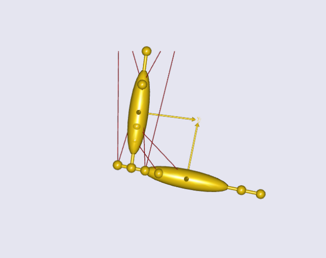
For us to do so, we first need to setup an example model. The model is a 2D arm model comprised of an upper and lower arm segment, attached with 8 simple muscles (fig. 1). The model is constraint to only allow movement in the global x and y direction. This allows us to impose movements which resembles flexion and extension of the shoulder and elbow joint. Further, we want to show a general way of calculating the strength independent of the movement, we therefore set up four load scenarios to mimic a flexion, extension, push, and pull movement.

Since we want to investigate maximum strength, we need to be sure that the muscles are recruited appropriately. This is done by switching to the MinMax_Strict muscle recruiter in the study section of our model. For more information on muscle recruitment in the Anybody Modelling software, se this tutorial.

The first step in finding the default maximum strength for a posture, is to know the relationship between load and MaxMuscleActivity ( \(m_{act}\) ). We can do this by implementing a parameter study to investigate the \(mmact\) across a spectrum of loads. This is done using the AnyParamStudy class as seen below:

  AnyParamStudy StrengthEval = 
  {
    Analysis = {AnyOperation& Opr = ..ArmStudy.InverseDynamics;}; 
    nStep = {100};

    AnyDesVar load = 
    {
      Val = Main.ArmModel.Loads.Dumbbell.load;
      Min = 0;
      Max = 250;
    };

    AnyDesMeasure maxact = 
    {
      Val = max(Main.ArmStudy.MaxAct());
    };
  };

This study runs our model through the loads defined in the \(load\) variable. So, in this example it does 100 steps where it starts at 0 N and stops at 250 N. This enables us to plot the \(m_{act}\) as a function of the load. By running the parameter study for all four load scenarios we end up with a graph as seen in fig. 2.

Fig. 2: Max muscle activity as a function of the applied load. Dashed line indicate $$mmact = 1$$.

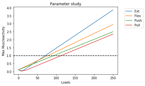
We can see that for very low loads there might be other factors than the applied load affecting the relationship. If we dwell by this fact and wonder why this could be, we could infer that the influence of gravity and segment mass could interfere with the relationship between \(load\) and \(m_{act}\). This means that when applying low external loads, the important factor in \(m_{act}\) is the mass of the moved segments, and the gravity imposed on those segments.

The graphs on fig. 2 also tells us that for high loads there is a linear relationship between load and \(m_{act}\), and the linear part is crossing $m_{act} = 1$ for all scenarios. We can use this information to calculate the maximum strength of the model. If we look at the equation for a linear function it looks like this:

\[\begin{equation} \label{eq:1} m_{act} = a * load + \ b \end{equation}\]

Where \(a\) is the slope of the function, and \(b\) is the intercept with the y-axis. The slope of the linear part can be calculated using only two points and applying the equation:

\[\begin{equation} \label{eq:2} a = \frac{(m_{act_{2}} - m_{act_{1}})}{(load_{2} - load_{1})} \end{equation}\]

Now that we know the coordinates of two points and the slope, we can start figuring out what the load is for an activity of 1 ( \(m_{act} = 1\) ). For this we again look at equation \(\eqref{eq:2}\), only this time we know the slope, the point $(load_{1},m_{act_{1}})\(, and the\)m_{act}$ coordinate, which should be equal to 1. We are therefore interested in finding the corresponding $load_{max}\(. We rearrange equation\)\eqref{eq:2}$, into:

\[\begin{equation} \label{eq:3} load_{max} = \frac{1}{a} - \frac{m_{act_{1}}}{a} + load_{1} \end{equation}\]

This allows us to evaluate what the maximum load \(load_{max}\) is, that the model can support for a given posture. To check our results, we can calculate the maximum strength for our four scenarios using equation \(\eqref{eq:3}\) and try to implement the output load in our models. Table 1. shows the calculated strengths of the models, and the \(m_{act}\) when applying the \(load_{max}\) values.

Movement	\(Load_{max}\) (N)	New \(m_{act}\)
Extension	70.97891372	1.0
Flexion	78.33099967	1.0
Push	93.43104145	1.0
Pull	113.1664796	1.0

Table 1: Calculated \(load_{max}\) and new \(m_{act}\) for each movement.

Now we can calculate the maximum load for any given posture!

Find the code on GitHub

The AnyScript example which shows the concept of finding the maximum strength is available on GitHub.