
Lesson 4: Parameter identification#
In this lesson we shall consider a source of uncertainty on motion capture experiments and musculoskeletal modeling in general that is completely different from the noise of the preceding section.
The issue is that a musculoskeletal model contains assumptions about the model dimensions that we really cannot know in advance. A femur, for instance, is attached to the hip joint located rather deeply inside the lower abdomen and we cannot palpate it or measure its location without advanced imaging techniques.
For a musculoskeletal model of a given individual, properties as basic as the length of the femur and the location of the hip joint center are always somewhat uncertain. In this section, we are going to see how the data in a C3D file can help us automatically determine these parameters with good accuracy.
Please download and save the file
multiple.c3d.
Then close all open windows in AnyBody and create a new Main file by
clicking the ‘M’ tool button in the upper left hand corner of the main
frame. This give you a dialog to create an empty model into which you can insert an
AnyInputC3D object, refer to the multiple.c3d file and specify the
filter as we did before:
Main = {

  // The actual body model goes in this folder
  AnyFolder MyModel = {
    // Global Reference Frame
    AnyFixedRefFrame GlobalRef = {
    // Todo: Add points for grounding of the model here
    };  // Global reference frame

    AnyInputC3D C3D =
    {
      FileName = "multiple.c3d";
      //ReadAllDataOnOff = On;
      //TruncateExtraCharsInNamesOnOff = On;
      //MakeNameUniqueStr = "_";
      //PointsScaleFactor = 1.0;
      //ConstructModelOnOff = On;
      ConstructChartOnOff = Off;
      //ConstructWeightFunUsingResidualOnOff = Off;
      //GapFillUsingResidualsOnOff = Off;
      //MarkerUseAllPointsOnOff = Off;
      //MarkerUseCamMaskOnOff = On;
      //MarkerIndices = ;
      //MarkerLabels = ;
      //MarkerFilterIndex = 0;
      //ProcessedDataFilterIndex = 0;
      //AnalogFilterIndex = -1;
      Filter =
      {
        AutomaticInitialConditionOnOff = On;
        FilterForwardBackwardOnOff = On;
        N = 2;
        Fc = {3};
        Type = LowPass;
      };
      //WeightThreshold = 0.0;
      //WeightOutput = {{0.0, 1.0}, {0.0, 1.0}, {0.0, 1.0}};
      //WeightTransitionTime = 0.1;
      //SearchAndReplace = ;
      //WriteMarkerDataToFilesOnOff = Off;
      //MarkerScaleXYZ = {0.025, 0.025, 0.025};
      MarkerRGB = {0, 0, 1};
      //MarkerDrawOnOff = On;
      //MarkerInterPolType = Bspline;
      //MarkerBsplineOrder = 4;
    };
Notice that we have also colored the markers blue with the MarkerRGB
property and disabled the plot of the 3D trajectories with the
ConstructChartOnOff property. We also set the duration of the movement
to automatically fit the C3D file as we have done before:
// The study: Operations to be performed on the model
AnyBodyStudy MyStudy = {
  AnyFolder &Model = .MyModel;
  Gravity = {0.0, -9.81, 0.0};
  AnyIntVar FirstFrame = Main.MyModel.C3D.Header.FirstFrameNo;
  AnyIntVar LastFrame = Main.MyModel.C3D.Header.LastFrameNo;
  tStart = FirstFrame/Main.MyModel.C3D.Header.VideoFrameRate+2*Kinematics.ApproxVelAccPerturb;
  tEnd = LastFrame/Main.MyModel.C3D.Header.VideoFrameRate-2*Kinematics.ApproxVelAccPerturb;
};
Now you should be able to load and run the model and see three blue markers travel through space in a motion that bears some resemblance to a football kick. The three markers are located on the same segment, and we happen to know that this segment is hinged in its upper end just like the pendulum in the previous lesson, but we do not know exactly where.
Three markers per segment are typical for many motion capture marker protocols. A segment with no other constraints, i.e. floating freely in space, has six degrees of freedom.
Although each marker provides three constraints, two markers are not enough to determine the location of the segment uniquely. The subtle explanation is that the markers are not independent because they are located on the same segment and therefore have their mutual distance given. In short, three non-collinear markers is the minimal set necessary to determine the location in space of an otherwise unconstrained segment.
Three markers then provide a total of nine constraints where the segment only has six DoFs, and the additional information from these markers can be used to determine other unknown factors in the model.
Let us initially define a segment and some guesses of where the three markers may be located on it:
Main = {

  // The actual body model goes in this folder
  AnyFolder MyModel = {
    // Global Reference Frame
    AnyFixedRefFrame GlobalRef = {
      // Todo: Add points for grounding of the model here
    };  // Global reference frame

    AnySeg Leg = {
      Mass = 1;
      Jii = {1, 0.01, 1}/15;
      AnyRefNode R1 = {
        sRel = {0.038, 0.18, 0.022};
      };
      AnyRefNode R2 = {
        sRel = {-0.015, -0.104, 0.028};
      };
      AnyRefNode R3 = {
        sRel = {-0.022, -0.403, -0.023};
      };
      AnyDrawSeg drw = {};
    };

    AnyInputC3D C3D =
    {
      FileName = "multiple.c3d";
Now we just need to use AnyKinDriverMarker objects to tie the marker trajectories to the three points we have defined on the segment and select the solvers for over-determinate problems exactly as we did in the previous lesson (don’t forget to also select the over-determinate kinematics solver in the study section):
  AnyKinDriverMarker C3Dmotion1 = {
    AnyRefFrame &Marker = .Leg.R1;
    AnyParamFun &Trajectory=
    Main.MyModel.C3D.Points.Markers.L000.PosInterpol;
    AnyDrawKinMeasure drw = {
      Label = Off;Size = 0.03;Line = Off;
    };
  };
  AnyKinDriverMarker C3Dmotion2 = {
    AnyRefFrame &Marker = .Leg.R2;
    AnyParamFun &Trajectory =
    Main.MyModel.C3D.Points.Markers.L001.PosInterpol;
    AnyDrawKinMeasure drw = {
      Label = Off;Size = 0.03;Line = Off;
    };
  };
  AnyKinDriverMarker C3Dmotion3 = {
    AnyRefFrame &Marker = .Leg.R3;
    AnyParamFun &Trajectory =
    Main.MyModel.C3D.Points.Markers.L002.PosInterpol;
    AnyDrawKinMeasure drw = {
      Label = Off;Size = 0.03;Line = Off;
    };
  };
}; // MyModel

// The study: Operations to be performed on the model
  AnyBodyStudy MyStudy = {
    AnyFolder &Model = .MyModel;
    Gravity = {0.0, -9.81, 0.0};
    AnyIntVar FirstFrame = Main.MyModel.C3D.Header.FirstFrameNo;
    AnyIntVar LastFrame = Main.MyModel.C3D.Header.LastFrameNo;
    tStart = FirstFrame/Main.MyModel.C3D.Header.VideoFrameRate+2*Kinematics.ApproxVelAccPerturb;
    tEnd = LastFrame/Main.MyModel.C3D.Header.VideoFrameRate-2*Kinematics.ApproxVelAccPerturb;
    InitialConditions.SolverType = KinSolOverDeterminate;
    Kinematics.SolverType = KinSolOverDeterminate;
  };
Now that we have created the AnyDrawKinMeasure objects, it is no longer necessary to have the points drawn in the C3D object. So let us get rid of them:
AnyInputC3D C3D =
{
  FileName = "multiple.c3d";
  //ReadAllDataOnOff = On;
  //TruncateExtraCharsInNamesOnOff = On;
  //MakeNameUniqueStr = "_";
  //PointsScaleFactor = 1.0;
  ConstructModelOnOff = Off;
  ConstructChartOnOff = Off;
  //ConstructWeightFunUsingResidualOnOff = Off;
  //GapFillUsingResidualsOnOff = Off;
  //MarkerUseAllPointsOnOff = Off;
It is now possible to run the Kinematics operation and see the leg segment move with the markers. The actual markers are not visible because they disappear inside the segment, but if we make the segment semi-transparent, they become visible:
AnySeg Leg = {
  Mass = 1;
  Jii = {1, 0.01, 1}/15;
  AnyRefNode R1 = {
    sRel = {0.038, 0.18, 0.022};
  };
  AnyRefNode R2 = {
    sRel = {-0.015, -0.104, 0.028};
  };
  AnyRefNode R3 = {
    sRel = {-0.022, -0.403, -0.023};
  };
  AnyDrawSeg drw = {
    Opacity = 0.5;
  };
};
We will also add a a drawing for the global reference frame, to better visualize the movement.
AnyFixedRefFrame GlobalRef = {
   AnyDrawRefFrame drw = {};
};
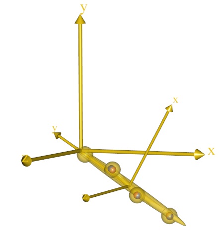
The animation reveals that the leg seems to rotate about the origin of the global reference frame, although we have not explicitly defined any joint. The point must obviously correspond to some point on the leg segment, but we do not know exactly where that is.
Let us define a joint point at an approximate location on the leg:
AnySeg Leg = {
  Mass = 1;
  Jii = {1, 0.01, 1}/15;
  AnyRefNode Joint = {
    sRel = {0, 0.45, 0};
  };
  AnyRefNode R1 = {
    sRel = {0.038, 0.18, 0.022};
  };
  AnyRefNode R2 = {
    sRel = {-0.015, -0.104, 0.028};
  };
  AnyRefNode R3 = {
    sRel = {-0.022, -0.403, -0.023};
  };
  AnyDrawSeg drw = {Opacity = 0.5;};
};
If you reload and re-run the model, you will see that the new point is approximately but not exactly the point the leg appears to rotate about. We could probably improve the location manually, but let us accept the location for now.
The next step is to create a revolute joint between the new point and the origin of the global reference frame:
AnyRevoluteJoint Joint = {
  AnyRefFrame &Ground = .GlobalRef;
  AnyRefFrame &Pendulum = .Leg.Joint;
};

AnyInputC3D C3D =
{
  FileName = "multiple.c3d";
A reload and re-run will reveal that the point is now forced to coincide
exactly with the origin of the coordinate system. This is because, as
opposed to AnyKinDriverMarker objects, joints by default contain hard
constraints that must be exactly fulfilled. The consequence is that the
blue marker dots inside the leg segment points now seem to deviate a bit
further from the center of the points.
There seems to be some unknown location of the joint center on the leg and possibly also of the marker points on the segment that we could either find by experimenting manually with the local coordinates of the points on the leg segment or, alternatively, ask AnyBody to find for us.
We are going to do the latter, and we shall employ a special study that
AnyBody has implemented for the purpose. Please click on the Classes tab
in the Tree View on the right side of the screen, expand the
Class List, and scroll down to find the AnyOptKinStudy. Place the cursor
after the end brace of the existing AnyBody Study, right-click the
AnyOptKinStudy in the Class Tree, and insert a template of the class:
// The study: Operations to be performed on the model
  AnyBodyStudy MyStudy = {
    AnyFolder &Model = .MyModel;
    Gravity = {0.0, -9.81, 0.0};
    AnyIntVar FirstFrame = Main.MyModel.C3D.Header.FirstFrameNo;
    AnyIntVar LastFrame = Main.MyModel.C3D.Header.LastFrameNo;
    tStart = FirstFrame/Main.MyModel.C3D.Header.VideoFrameRate+2*Kinematics.ApproxVelAccPerturb;
    tEnd = LastFrame/Main.MyModel.C3D.Header.VideoFrameRate-2*Kinematics.ApproxVelAccPerturb;
    InitialConditions.SolverType = KinSolOverDeterminate;
    Kinematics.SolverType = KinSolOverDeterminate;
  };
  AnyOptKinStudy <ObjectName> =
  {
    //LogFile = "";
    /*Analysis =
    {
    Settings =
    {
    Echo = On;
    ModelSceneUpdate = On;
    };
    //AnyOperation &<Insert name0> = <Insert object reference (or full object definition)>; You can make any number of these objects!
    };*/
    //MaxIterationStep = 100;
    AnyDesMeasure &<Insert name0> = <Insert object reference (or full object definition)>;
    //AnyDesMeasure &<Insert name1> = <Insert object reference (or full object definition)>; You can make any number of these objects!
    //AnyDesVar &<Insert name0> = <Insert object reference (or full object definition)>; You can make any number of these objects!
  };
The AnyOptKinStudy’s structure is very similar to the general optimization
class AnyOptStudy, but it contains an algorithm specially made for kinematic
parameter optimization and several of the necessary definitions are implicit, so
the study is simple to use. All we have to do is to specify the unknown
parameters in the model and the location of the kinematic analysis necessary to
evaluate them.
We begin with the latter and make the following changes:
AnyOptKinStudy OptKinStudy =
{
  Analysis = {
     AnyOperation &Operation= ..MyStudy.Kinematics;
  };
  //MaxIterationStep = 100;
  AnyDesMeasure &<Insert name0> = <Insert object reference (or full object definition)>;
};
Now we have specified that we want to optimize parameters to fit the experimental data used in the Kinematics analysis of the original study, i.e. the C3D data.
The next step is to specify which parameters to
optimize. In this case, we are uncertain about the precise location of
the revolute joint in the upper end of the segment. Its location is
defined by the local coordinates to the AnyRefNode ‘Joint’ on the leg
segment:
AnyOptKinStudy OptKinStudy =
{
  Analysis = {
     AnyOperation &Operation= ..MyStudy.Kinematics;
  };
  //MaxIterationStep = 100;
  AnyDesVar Jointx = {
    Val = Main.MyModel.Leg.Joint.sRel[0];
  };
};
This specifies that the zero’th coordinate, i.e. the local x coordinate of the Joint node on the Leg segment is a variable in the problem.
Similarly, we can add the y and z coordinates:
AnyOptKinStudy OptKinStudy =
{
  Analysis = {
     AnyOperation &Operation= ..MyStudy.Kinematics;
  };
  //MaxIterationStep = 100;
  AnyDesVar Jointx = {
    Val = Main.MyModel.Leg.Joint.sRel[0];
  };
  AnyDesVar Jointy = {
    Val = Main.MyModel.Leg.Joint.sRel[1];
  };
  AnyDesVar Jointz = {
    Val = Main.MyModel.Leg.Joint.sRel[2];
  };
};
Now we can reload the model and a new set of operations will have appeared:
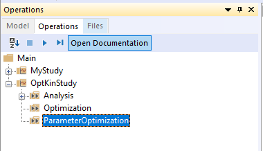
Pick the ParameterOptimization and click the Run button.
If you have a Model View open, you will see the pendulum starting to move and messages about the convergence of the process will appear in the Report View at the bottom of the screen.
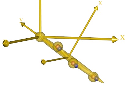
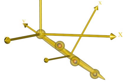
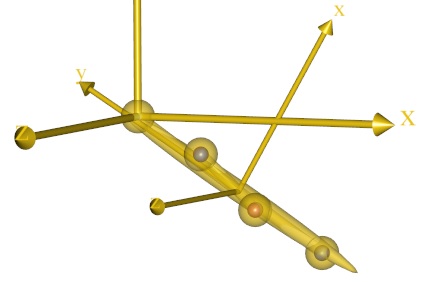
Pay close attention to the location of the small blue markers inside the larger yellow dots on the segment. The blue dots should move considerably closer to the centers of the yellow balls as a consequence of the optimization as shown below, where the left picture is the location of the markers before the joint location optimization, and the right picture shows the situation after optimization.
This notion is confirmed by opening opening the chart view and plotting the development of the objective function of the problem:
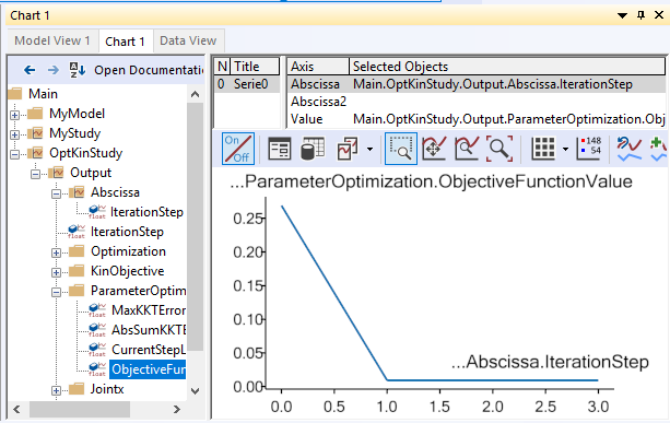
The graph shows that the norm of the difference between the measured marker positions and the corresponding nodes on the segment over the entire motion was reduced from about 0.27 to about 0.01.
Now that we have identified a better location of the joint node on the segment, we might want to save it for later use.
This is done by right-clicking the OptKinStudy in the operations tree on the
left hand side of the mainframe and selecting “Save design” from the context
menu. This opens a file manager dialogue. Please navigate to the directory where
you keep the model and specify a name for the new file, for instance
Opt1.txt.
If you open the new file you can see the saved values:
Jointx 1.574794116583949e-002
Jointy 4.907819352974447e-001
Jointz 6.507036792142549e-004
You can easily load these values into your model from the same context menu every time you have reloaded the model.
Of course, to have the coordinates of the Joint node permanently updated, you can also simply copy and paste them into the sRel value directly in the Leg segment definition in your AnyScript file. Don’t do it yet, though. We are going to play a little more with the possibilities.
The optimization we have just completed has presumed that we know well where the markers are located on the segment but are in doubt about the location of the joint, such as would often be the case in a gait analysis involving a hip joint.
However, even if we use a marker protocol that places most markers on well-defined bony landmarks in the model, there may still be doubt about the precise locations of some or all the markers, and the result of the joint location optimization also shows that especially the first marker location deviates somewhat from its corresponding AnyRefNode. This indicates that there are other sources of error in the model, than the joint location, and indeed the recent relocation of the joint may be influenced by errors that are not associated with the joint location.
This is the reason why it was advised to not permanently update the joint location. When the optimization is redefined to also comprise the marker positions. It is better to simultaneously optimize the joint position and marker locations.
The marker node position is included in the optimization in the same way as the Joint node:
AnyOptKinStudy OptKinStudy =
{
  Analysis = {
     AnyOperation &Operation= ..MyStudy.Kinematics;
  };
  //MaxIterationStep = 100;
  AnyDesVar Jointx = {
    Val = Main.MyModel.Leg.Joint.sRel[0];
  };
  AnyDesVar Jointy = {
    Val = Main.MyModel.Leg.Joint.sRel[1];
  };
  AnyDesVar Jointz = {
    Val = Main.MyModel.Leg.Joint.sRel[2];
  };
  AnyDesVar R1x = {
    Val = Main.MyModel.Leg.R1.sRel[0];
  };
  AnyDesVar R1y = {
    Val = Main.MyModel.Leg.R1.sRel[1];
  };
  AnyDesVar R1z = {
    Val = Main.MyModel.Leg.R1.sRel[2];
  };
Please reload and re-run the Main.OptKinStudy.ParameterOptimization.
Note
To speed up the optimization study, try to disable Model View by clicking the “On/Off” button in the Model view toolbar.
The convergence should be quite fast in such a small model, and you arrive at the following solution:
The solution appears to be bull’s eye in terms of placing the markers in the center of the yellow nodes. This is confirmed by the optimized value of the objective function: the residual of the distance between markers and nodes is now less than 0.001.
It appears that we have obtained an almost perfect solution, but why not include all the marker nodes in the optimization? Well, we can try adding another one:
AnyOptKinStudy OptKinStudy =
{
  Analysis = {
     AnyOperation &Operation= ..MyStudy.Kinematics;
  };
  //MaxIterationStep = 100;
  AnyDesVar Jointx = {
    Val = Main.MyModel.Leg.Joint.sRel[0];
  };
  AnyDesVar Jointy = {
    Val = Main.MyModel.Leg.Joint.sRel[1];
  };
  AnyDesVar Jointz = {
    Val = Main.MyModel.Leg.Joint.sRel[2];
  };
  AnyDesVar R1x = {
    Val = Main.MyModel.Leg.R1.sRel[0];
  };
  AnyDesVar R1y = {
    Val = Main.MyModel.Leg.R1.sRel[1];
  };
  AnyDesVar R1z = {
    Val = Main.MyModel.Leg.R1.sRel[2];
  };
  AnyDesVar R2x = {
    Val = Main.MyModel.Leg.R2.sRel[0];
  };
  AnyDesVar R2y = {
    Val = Main.MyModel.Leg.R2.sRel[1];
  };
  AnyDesVar R2z = {
    Val = Main.MyModel.Leg.R2.sRel[2];
  };
When you reload the model and re-run the ParameterOptimization, you will find that the optimization takes much more time, the convergence is much less stable, the segment moves far away from the marker nodes in the process, and eventually the algorithm gives up with the error message:
Optimization failed : Failed to solve position analysis
You can understand the reason for this behavior if you look at the figure of the previous result above and imagine that we make all four visible points variable, i.e. in a sense cut them loose from the segment in the optimization problem. Then the segment can float freely in space while the nodes are free to fall exactly on top of their respective markers and the joint at the origin of the global reference frame.
In other words, such a problem has infinitely many perfect solutions and the location of the segment cannot be determined from the optimization problem. In other words, for a problem like this to be well-posed, some points have to be fixed.
When we add the second marker position to the optimization problem, we leave the model with only two fixed nodes, namely the third marker node and the joint node. This leaves the segment the opportunity to rotate freely about an axis through the two fixed points, and the optimization problem is ill-posed because it does not determine the rotation of the segment.
Obviously, in a practical case you would select as the invariable marker nodes those that are physiologically well-determined, for instance from easily accessible bony landmarks.
Hopefully, this simple, bottom-up example has demonstrated how the technology works.
Now, let us change our focus to a top-down approach and see what the technology can do with real motion capture data. That will be the subject of Lesson 5.