
Lesson 3: Kinematic Analysis#
The Kinematics operation can be explained in two ways: a brief overview and a
detailed deep dive. The brief overview is that it enables your model to execute
the movements you’ve defined using drivers, focusing solely on the movement
without involving any force calculations. Even if the system isn’t perfectly
balanced, it can still undergo the Kinematics operation. However, the model
must be kinematically determinate, a concept we’ll explore in the detailed
explanation.
So, get ready, and let’s dive deeper into…
The long explanation – tl;dr
An AnyBody model is essentially a collection of rigid segments, which you can visualize as potatoes floating in space. In the context of AnyBody, we refer to these “rigid bodies” as “segments”. The physics term “rigid body” is called a “segment” in AnyBody to avoid confusion with the layman/physiological term for “body”.
Each segment can move in six different directions, or degrees of freedom: three movements along the coordinate axes and three rotations about the same axes. If we have \(n\) segments in the model, the model will have a total of \(6n\) degrees of freedom, unless some are constrained. The goal of kinematic analysis is to determine the position of all segments at all times, which requires \(6n\) pieces of information, or equations, to resolve the \(6n\) degrees of freedom.
One common way to constrain degrees of freedom (or add equations) is to add joints to the model. When two segments are joined, they lose some of their freedom to move independently. For example, two segments joined at their ends by a ball-and-socket joint are constrained such that the \(x\), \(y\), and \(z\) coordinates of the joined points must be the same, adding three constraints or equations to the system.
If you add enough joints to provide all \(6n\) constraints, it might be mathematically possible to solve the equations and find the position of all the segments. However, the result would be static, as the system would not be able to move. Typically, a body model will have enough joints to keep the segments together but few enough to allow the model to move. The remaining constraints or equations come from the drivers. After the joints have consumed their share of the degrees of freedom, enough drivers must be added to resolve the remaining unknowns in the system up to the required number of \(6n\). During the Kinematics operation, these drivers are taken through their sequences of values, and the positions of all the segments are resolved for each time step by solving the \(6n\) equations.
A model is said to be kinematically determinate when it has \(6n\) equations that can be solved. This is usually necessary for the kinematic analysis. However, there are exceptions where the system can be solved even when the number of equations differs from \(6n\), or when the system cannot be solved even though there are \(6n\) equations available. Both cases involve redundant constraints.
Redundant constraints are those that constrain the same degrees of freedom in the same way. For example, if you accidentally define a joint twice, the equations provided by those two joints will be redundant. They will appear when you count constraints, but they won’t have much effect.
The AnyBody Modeling System can sometimes handle models with too many constraints, as long as those constraints are not conflicting, i.e., some of them are redundant. However, it’s a good practice to ensure that the number of degrees of freedom matches the number of constraints.
If you have too many conflicting constraints, the system is kinematically over-determinate. If you have too few constraints, or some of the constraints are redundant, the system may be kinematically indeterminate. Both cases are likely to prevent the Kinematics operation from completing.
Even with a kinematically determinate system, the Kinematics operation can fail. This can occur when the segments of the model are configured such that they cannot reach each other, or they interlock. Real-world examples include car doors that get stuck or refuse to close, locks that won’t unlock, or stacked glasses that wedge inseparably into each other. Computer systems that model the real world will have similar issues, and just like in the real world, it can sometimes be difficult to identify the problem.
Running a Kinematic Analysis#
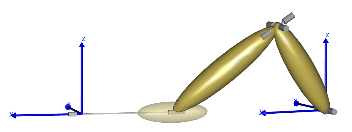
In this section, we’ll delve into the process of performing a kinematic analysis. To illustrate this, we’ll use the following example:
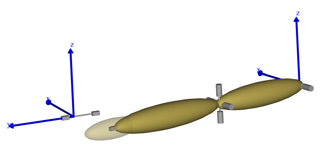
Upon loading the demo.SliderCrank3D.any file and examining the Model View, you’ll notice a simple mechanism consisting of three segments. Initially, these segments are not correctly connected at their joints. However, running the Kinematics operation will rectify this, resulting in a fully assembled and operational model.
The Kinematics operation is essentially an analysis tool. It stores data during its run, allowing you to explore the results in the Chart view. The data you can extract from the Kinematics study includes positions, velocities, and accelerations.
To view these results, expand the tree until you reach the Slider segment. Here, you can chart its acceleration by selecting the rDDot property.
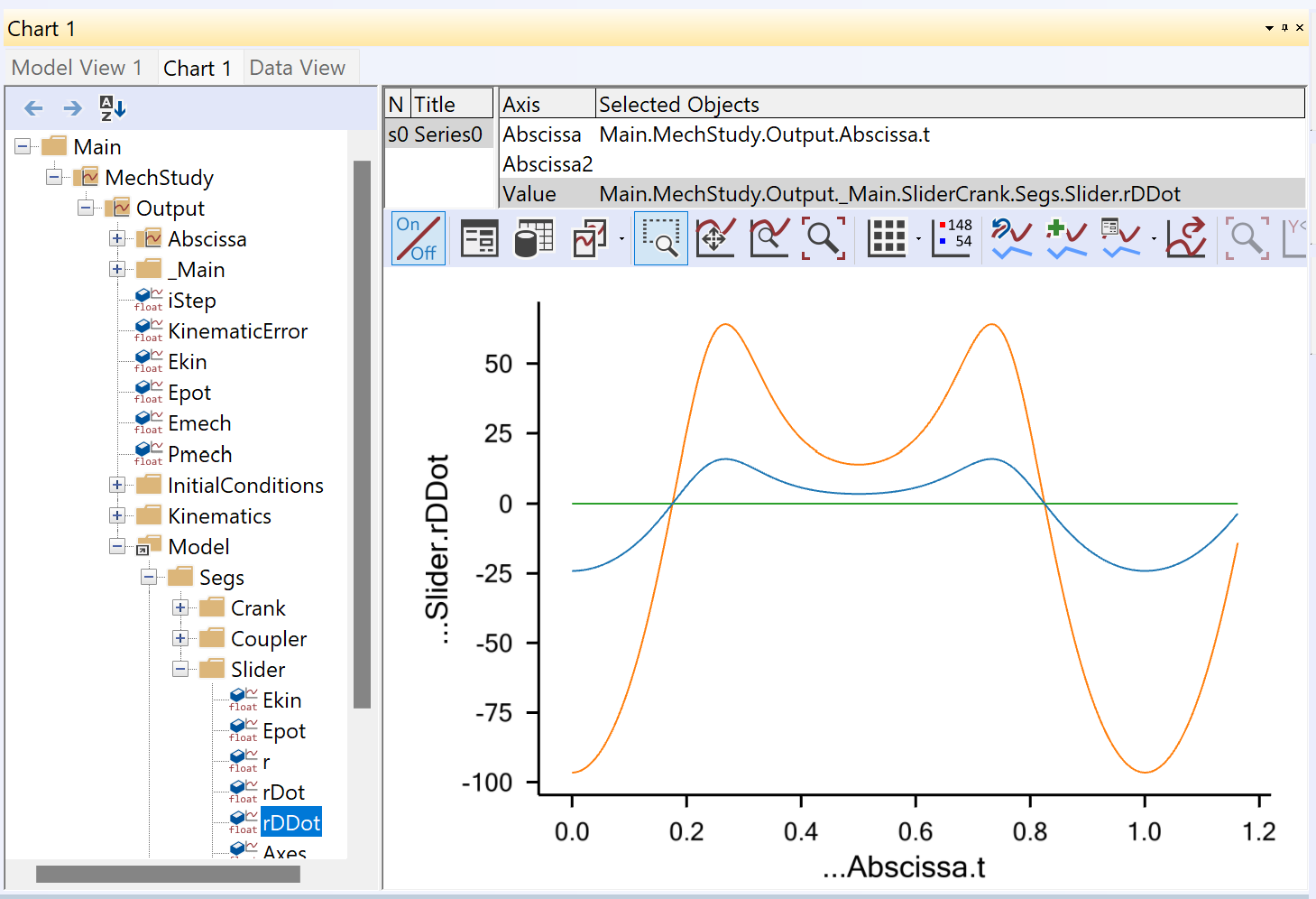
Take note of how the positional properties are named: r stands for position, rDot for velocity, and rDDot for acceleration. The terms “Dot” and “DDot” are derived from mathematical conventions, where a dot above a symbol indicates differentiation with respect to time. Hence, velocity is represented as \(\dot{r}\), and acceleration as \(\ddot{r}\). Feel free to explore the tree and familiarize yourself with the various data available.
You might come across some results that seem unusual, like the one below:
You might be wondering why a smoothly running model would show such behavior. The key to understanding this lies in the y-axis. Notice that the values are around 1e-14, which is essentially zero. What you’re seeing here is not a significant value, but rather, it’s zero affected by tiny numerical rounding errors.
Final remarks#
👉 Remember, kinematic analysis doesn’t just find positions, it also calculates velocities and accelerations. Figuring out the positions is the trickiest part because it involves nonlinear equations. Once we have the positions, finding velocities and accelerations is easier because we’re dealing with linear equations.
One of the unique things about the AnyBody Modeling System is its ability to handle closed kinematic chains. This is super important in biomechanics, where these chains pop up all the time. Think about activities like cycling, walking, or grabbing an object with both hands.
While kinematic analysis is a powerful tool on its own, it’s also the first step in the InverseDynamics operation. We’ll dive into that in our next lesson.