
Lesson 1: Export of Data for FEA#
In this example, we aim to address an important issue for aquarium owners: What is the magnitude of stress in the lumbar vertebra L5 during the lifting of a 10 kg aquarium?
First, we need a model to work on.
With the AnyBody Modeling System, you already have a repository of models available. For details, please see the AnyBody Assistant available from the menu. This tutorial was written using the AnyBody Managed Model Repository Version 4 (AMMRV4) and will not work on earlier versions. If you notice differences between the tutorial text and your results, please report or help fix it here.
The starting point for this tutorial is the model:
Applications/Examples/StandingLift/StandingLiftFEA.main.any
However, this model internally reuses the code of StandingLift.main.any.
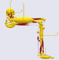
Please find the model and load it by pressing F7, and open a Model View. You
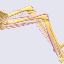
should see something similar to the picture above. The vertebral body we want to
analyze is marked with a square in the zoomed-in picture.
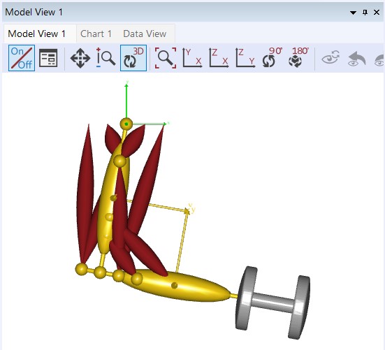
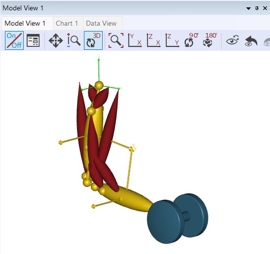
As mentioned before, this model is based on the “StandingLift” model of the AMMR
4 Repository. It is a full-body model lifting a box of 10 kg and therefore also
imposing forces on the spine. In this tutorial, we simplify by only using the
model with joint generating muscles; this will keep the force output files
small. Go to StandingLift.main.any -> Model/BodyModelConfigurationFEA.any to
see the code applying this simplification.
// switch the muscles off for simplicity
#define BM_LEG_MUSCLES_RIGHT OFF
#define BM_LEG_MUSCLES_LEFT OFF

#define BM_ARM_MUSCLES_RIGHT OFF
#define BM_ARM_MUSCLES_LEFT OFF

#define BM_TRUNK_MUSCLES OFF
By default, this model uses a simplified version of the vertebra L5, which we
don’t want to use for our finite element analysis. Therefore, we will comment
out the following lines of code in StandingLift.main.any:
// #ifdef FEA_OUTPUT
  // this block replaces an intact L5 geometry with a simplified one
  // #include "Model/L5Modifications.any"
// #endif
Exporting the Forces#
To export the forces acting on the vertebra, we had to include the output function. This modification can be found inside the Study folder of the main file:
#ifndef FEA_OUTPUT
// default values for the StandingLift example
  tEnd = 1.0;
  nStep = 30;
#else
// single step for the StandingLiftFEA example
  tStart = 0.5;
  tEnd = 0.5;
  nStep = 1;
  AnyMechOutputFileForceExport ForceOutput =
  {
    FileName = ANYBODY_PATH_OUTPUT+"/ForceL5.txt";
    /*NumberFormat =
    {
    Digits = 15;
    Width = 22;
    Style = ScientificNumber;
    FormatStr = "";
    };*/
    AllSegmentsInStudyOnOff = Off;
    Segments = {&Main.HumanModel.BodyModel.Trunk.Segments.L5Seg};
  };
#endif
The AllSegmentsInStudyOnOff switch decides if only the forces of the listed
segments will be exported or data from all segments in the study. Usually, you
will only use a selected amount of data to keep the file manageable. The
following segment points to the L5 segment, which is the one we want to analyze.
If the path is not already inserted, you can fill in the path by browsing the
Model tab to the L5 segment, right-clicking it, and choosing “Insert Object
Name” in the drop-down menu.
That’s all we have to do for the force export. Please reload the model by pressing F7 and run an “InverseDynamicsAnalysis”. The model will analyze one timestep and write the “ForceL5.txt” file which we have specified earlier. Let’s take a closer look at the output file. It is located inside your Application folder in the Output subfolder. You can open it either directly in AnyBody or in any text editor of your choice.
Environment:
ReferenceFrame=Global Model Frame;
Gravity=  0.000000000000000e+00; -9.810000000000000e+00;  0.000000000000000e+00;

Segments(1):
Segment[0] type="string" value="Main.HumanModel.BodyModel.Trunk.Segments.L5Seg":
AMesh=  1.000000000000000e+00,  0.000000000000000e+00,  0.000000000000000e+00;  0.000000000000000e+00,  1.000000000000000e+00,  0.000000000000000e+00;  0.000000000000000e+00,  0.000000000000000e+00,  1.000000000000000e+00;
rMesh=  0.000000000000000e+00;  0.000000000000000e+00;  0.000000000000000e+00;


TimeSamples:
===================== Start of time-step =====================
TimeSample[0]:
t=  5.000000000000000e-01;
Segment[0]:
Name=Main.HumanModel.BodyModel.Trunk.Segments.L5Seg;
m=  8.647575371435805e-02;
Jmatrix=  3.117695761957781e-05, -4.208528827168931e-05, -3.334400020792064e-14; -4.208528827168931e-05,  1.994722295336756e-04, -1.000086230663426e-14; -3.334400020792064e-14, -1.000086230663426e-14,  2.041147280980830e-04;
rCoM=  4.630659278707620e-02;  1.098979341331007e+00; -2.829688056260412e-04;
r=  1.625397040768109e-03;  1.090864811079046e+00; -9.334043002481586e-05;
Axes=  9.965798817571829e-01,  8.262426983257545e-02,  1.330154680284060e-03; -8.263497611084375e-02,  9.964507636492066e-01,  1.604170645765142e-02;  6.359913417306254e-10, -1.609675922497869e-02,  9.998704387781716e-01;
rDot=  8.556741311315945e-04; -1.165877289154847e-06;  4.581814730063425e-05;
Omega=  7.875404885864421e-03; -6.530172907226420e-04; -9.226347600732171e-04;
rDDot=  7.111300235124309e-03; -5.212047158521299e-05; -2.191805043600826e-03;
OmegaDot= -3.767377450842683e-01;  3.123123803534829e-02; -7.671516835546827e-03;

Forces(25):
Force[0]:
Name=Main.HumanModel.BodyModel.Trunk.JointMuscles.Lumbar.L5Sacrum.Extension.Object.Muscle.PosMuscle;
Class=AnyMainFolder.AnyFolder.AnyFolder.AnyFolder.AnyFolder.AnyFolder.AnyFolder.AnyFolder.AnyFolder.AnyFolder.AnyMuscleGeneric;
SegmentName=Main.HumanModel.BodyModel.Trunk.Segments.L5Seg;
SegmentID=0;
Pos=  4.535990497088651e-02;  1.081420529974129e+00;  3.881010741458354e-10;
RefFrame=Main.HumanModel.BodyModel.Trunk.Segments.L5Seg.L5SacrumJntNode;
Components(1):
F[0]=  0.000000000000000e+00;  0.000000000000000e+00;  0.000000000000000e+00;
M[0]= -3.045196940829644e-08;  6.444859431831559e-09;  4.854333671269095e+01;
...
The text file starts with information on the included segments, listing all geometrical entries in the global coordinate system. Following this, all forces acting on the segment are listed, including the position and components of each force from AnyBody. The underlying “Class” entry indicates the type of AnyForce, which can have various components. An AnyForce may have any number of components, which may be a physical force or a torque, but it may also be a more generalized load, not measured in Newtons or Newton-meters.
These force components are related to the underlying kinematic measure, meaning
force times kinematic displacement equals work/energy; in other words, the
kinematic measure determines the unit of the force component. These force
measures present in the Anybody model are converted to real point forces and
torques in the AnyFE output file, represented as F[i] and M[i]. These are
the point forces and the point torques associated with the i’th component of
the given AnyForce object. The total force acting in the global direction at any
given point is the sum of all F[i] components.
In many cases, the components are indeed simple such that component i=0 for
instance is Fx as could be expected. However, since this Fx may refer to a
local coordinate system of a particular segment, a joint attachment node, or the
like, F[i] and M[i] may still have three non-zero values when exported to
the AnyFE file. This is because the data is transformed while being exported so
that the AnyFE refers to a single coordinate system for all of the exported
data; this system is often (by default) the global coordinate system, but it can
also be a local coordinate system.
Let us have a look at the following entry which essentially provides the joint constraints in the L5-Sacrum joint:
Force[14]:
Name=Main.HumanModel.BodyModel.Trunk.Joints.Lumbar.L5Sacrum.Constraints.Reaction;
Class=AnyMainFolder.AnyFolder.AnyFolder.AnyFolder.AnyFolder.AnyFolder.AnySphericalJoint.AnyKinEq.AnyReacForce;
SegmentName=Main.HumanModel.BodyModel.Trunk.Segments.L5Seg;
SegmentID=0;
Pos=  4.535990497088651e-02;  1.081420529974129e+00;  3.881010741458354e-10;
RefFrame=Main.HumanModel.BodyModel.Trunk.Segments.L5Seg.L5SacrumJntNode;
Components(3):
F[0]= -3.976388673919678e+01;  3.297164523303544e+00; -2.538223591233220e-08;
M[0]=  0.000000000000000e+00;  0.000000000000000e+00;  0.000000000000000e+00;
F[1]=  3.959699254370243e+01;  4.775407219118766e+02; -3.856093434975321e-08;
M[1]=  0.000000000000000e+00;  0.000000000000000e+00;  0.000000000000000e+00;
F[2]= -4.017792322478466e-17;  8.503261775118913e-18;  6.404743251140932e-08;
M[2]=  0.000000000000000e+00;  0.000000000000000e+00;  0.000000000000000e+00;
You can see the three moments have zero values. This is because this joint is discretized as a spherical joint which therefore cannot take up moments. Similarly, all other joints are handled.
Exporting the Geometry#
Next, we need an object where we can apply our exported forces. This is also
quite simple. A facility is built in the system (from Version 3.1) which allows
the export of all .anysurf and .stl geometries from your application in the .stl
file format. The function will export the geometry in its actual position, so
please make sure that your model has not been reloaded since the force export.
Otherwise, run the InverseDynamicAnalysis again to bring it to the right
position. Of course, it also involves all scaling that has been applied to the
bones.
Browse through the model tree to the L5Seg under
Main/HumanModel/BodyModel/Trunk/Segments/L5Seg in order to export the L5
segment. Inside this folder, you find the BoneDraw folder. Right-click the
folder and choose “Export Surface”. Choose a convenient place to store the file
and give it the name “L5.stl”. A dialog box will appear that allows you to
specify a scaling factor for the output file. The scaling can be useful to
switch from one unit system to another. In our case, we have meters as units in
the AMS, but want to have millimeters for the FE geometry. So choose a scaling
factor of 1000. After clicking OK, a new dialog box will appear that allows you
to select a reference frame. Choose “Global” and click OK. From the AnyBody
point of view, that’s all we have to do.
Note
Please note that not all bones currently in the Repository may be
suitable for FEA. As the main intention is to have a graphical representation of
the body, it may appear that some bones are simply too coarse for a detailed
analysis. But of course, you are free to import your own .stl file into the
AnyBody Modeling System to substitute existing bones. You will have to tweak
your CAD file a bit in order to make it fit. Donation of better quality CAD
files of bones to the models is most welcome.
Based on the exported forces and .stl file we can now build and analyze a
finite element model. Below, we shall build an FE model by manually applying the
loads and other boundary conditions using non-commercially available software.
However, please note that in the following lessons, we consider more smooth
integration with selected commercial software by means of small converter
software tools provided by AnyBody Technology. These tools automatically convert
the AnyFE output file from AnyBody to input files for the particular FE
software.
After building an FE model based on this data, the stress in the bone tissue can be evaluated.
Building the Finite Element Model#
In this section, a short description of how to build a finite element model using AnyBody data is given. If you are an experienced FE user, you may want to skip this section.
As this is by no means a Finite Element tutorial, we will use some shortcuts to achieve our goal: We have already restricted the analysis to one time step. Further, we will only take the joint reaction forces into account.
In the following, we will make use of a freely available software, FEBio. This software can handle the preprocessing (meshing and applying boundary conditions), solve the FE analysis, and handle the post-processing of the FE model. Please note that this program is in no relation to AnyBody Technology.
Please follow the link shown above to download and install the program if you want to do some hands-on FEA.
Building the Model - Preprocessing#
A file with the finished model is provided below, in case you do not want to go through the entire model building process.
👉 Now Open FEBio and start a New Model. Select ‘Structural Mechanics’, give your model an appropriate name, e.g. “StandingLiftFE”, and select ‘mm-kg-s’ as the unit system.
To open the earlier exported .stl file of the geometry, select ‘Import
Geometry’ under File and browse to the location of your STL-file.
After successfully loading the geometry, we have to generate a mesh with solid elements. The geometry already has an initial mesh based on the STL-file, but we want to refine and specify it. This is done by first right-clicking on the name “L5-stl” in the Model Tree, choosing “Select” and clicking on the geometry in the model view. This opens the Build panel to the right where you can choose Mesh and convert Type to ‘Editable surface’, which allows us to change the mesh using solid elements.
Under Mesh Parameters set the Element Size to 6, the Quality to 2 and click Apply to generate an initial mesh using 4-node linear tetrahedral elements. To further specify the mesh, click on MMG Remesh under Edit Mesh. This is a tool to re-create the mesh or apply a local mesh refinement or coarsening of a mesh. Under parameters set Element size to 6, Min element size to 2, Global Hausdorff value to 0.05 and Gradation to 1.3. Click Apply to generate this new mesh.
One could go much further in the meshing process to optimize it, but for this example, this is sufficient.
Note
It may graphically appear that some parts of the geometry do not have a mesh or that the mesh suddenly disappears. This is due to the Global Hausdorff value, which allows for a distance between the surface of the generated mesh and the locally interpolated quadratic surface of the geometry.
After this, we have to assign material properties to the model. Right-click on Materials in the Model Tree, select ‘Add Material’ and choose ‘Isotropic elastic’ as the type. This adds a new material which we now can specify. Click on the newly added material to open the info tab. Reasonable values for bone material could be to set the Density to 1.3e-09 kg/mm^3, the Young’s modulus to 1e+06 kPa, and the Poisson’s ratio to 0.3. Under Geometry -> Objects -> L5.stl -> Parts click on Part1, and under Properties apply “Material 1” as the material.
The material selection used is an approximation of the real bone, but of course, you may also want to model the bone in more detail, separating the cortical shell and the cancellous bone or even basing the material properties on density data. But this is surely not within the scope of this tutorial.
In this example, we will apply only the joint reaction forces on the endplates. Therefore, we will not make explicit use of all the information given by the AnyBody force export file. We now have to select two sets of nodes to apply the boundary conditions.
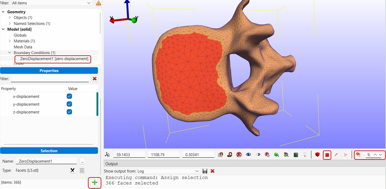
Start by right-clicking on Boundary Conditions in the Model Tree and selecting ‘Add Nodal BC’. Choose ‘Zero Displacement’ and under Property check out x-, y-, and z-displacement. Next, select an area of element faces on the bottom endplate, similar to the selection on the image below, to apply this boundary condition. To do this, click on the part in the model view, choose ‘Select faces’ and ‘Select connected’, both in the Graphics control bar (highlighted with a red square in the image below), and select an element face. It might be necessary to adjust the value for the ‘Select Connected’ option. If this does not automatically select all the wanted element faces, simply hold the shift button down while manually selecting multiple faces, or hold the control button down to deselect faces. Finally, add the selected faces by clicking the plus sign under Selection.
Now the force must be applied. For this, we need our force export file. Please open the file (it should be located in your StandingLiftFEA application folder) in an editor and scroll down to Force[14]. This force is the joint reaction on the L5-Sacrum joint.
Force[14]:
Name=Main.HumanModel.BodyModel.Trunk.Joints.Lumbar.L5Sacrum.Constraints.Reaction;
Class=AnyMainFolder.AnyFolder.AnyFolder.AnyFolder.AnyFolder.AnyFolder.AnySphericalJoint.AnyKinEq.AnyReacForce;
SegmentName=Main.HumanModel.BodyModel.Trunk.Segments.L5Seg;
SegmentID=0;
Pos=  4.535990497088651e-02;  1.081420529974129e+00;  3.881010741458354e-10;
RefFrame=Main.HumanModel.BodyModel.Trunk.Segments.L5Seg.L5SacrumJntNode;
Components(3):
F[0]= -3.976388673919678e+01;  3.297164523303544e+00; -2.538223591233220e-08;
M[0]=  0.000000000000000e+00;  0.000000000000000e+00;  0.000000000000000e+00;
F[1]=  3.959699254370243e+01;  4.775407219118766e+02; -3.856093434975321e-08;
M[1]=  0.000000000000000e+00;  0.000000000000000e+00;  0.000000000000000e+00;
F[2]= -4.017792322478466e-17;  8.503261775118913e-18;  6.404743251140932e-08;
M[2]=  0.000000000000000e+00;  0.000000000000000e+00;  0.000000000000000e+00;
By summing up the rows for the forces F[0], F[1], and F[2] we get the
resulting components for the joint reaction load. This can be directly used in
the force definition since they are given in the same coordinate system. In this
case, only the Y-force component is of interest as all other forces are small in
comparison when summing them up. Now right-click on Loads in the Model Tree and
select ‘Add Surface Load’ and choose ‘Force’ in the pop-up window. Set the Force
to {0, 517000, 0} mN and apply it to an area of element faces, similar to what
you did for the boundary condition selection, but on the opposite endplate.
Finally, we need to create an analysis step and change the load controller to define what type of analysis we want to do and how the loads are applied. Add an analysis step by selecting Physics -> ‘Add Analysis Step’ from the top menu and then click OK. Since we want to perform a static analysis, we keep all settings under Properties as they are. Now, expand Load Controllers, select the Load Controller LC1 in the model tree and under Properties make sure the ‘Type’ is set to ‘Linear’. (You should only have one Load Controller in the model. If you have more, delete the ones with an exclamation mark)
Solving and Post-Processing#
Congratulations! The model is now finished. Now we have to run and solve the FE model.
First, save the model if you have not already done so. Then, click on FEBio in the top menu and select ‘Run FEBio’. In the pop-up window define the Job name (could be “StandingLiftFE_RUN”), make sure the Launch Configuration is set to ‘Default’. Finally, click Run to start the analysis.
The analysis should only take a few seconds, and a pop-up window will appear when the analysis is finished. Here the Status should say ‘Normal Termination’ and Completion 100%. Click on ‘Open results’ to see the simulation outputs.
You now have many options to visualize the results. To learn more about the
FEBio post-processing go to the FEBio
Knowledgebase. One option is to plot the von
Mises stress in the model. To do this, click on Color Map in the Post menu.
Under Properties change Data Field to Stress -> Effective stress, Show Legend to
‘Yes’, and both Max range type and Min range type to ‘Static’. Now click the
Play button  in the top menu to show the
von Mises stress plot in the model.
in the top menu to show the
von Mises stress plot in the model.
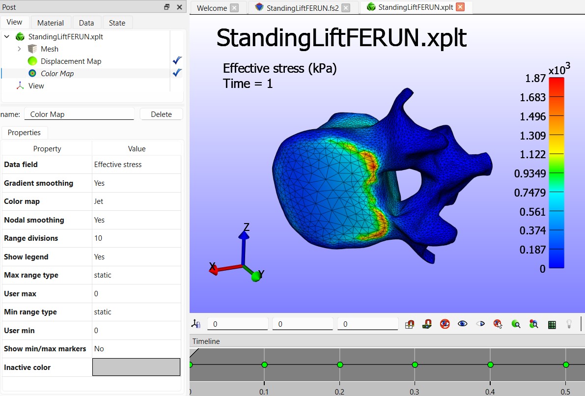
The above image shows the von Mises (effective) stress plot of the lumbar vertebra L5. With a maximum stress of approximately 1.87 MPa in the bone, we are far away from the yield strength. So, we can conclude that it appears to be ok for aquarium owners to lift their pets in an aquarium of this size. But of course, we did some generous shortcuts to achieve this goal and neglected a lot of detail which is provided by the AnyBody Modeling System.
This completes Lesson 1. The final FEBio model and AnyBody script can be
downloaded here. It is important that
you place it in a folder containing the AMMR 4 ‘libdef.any’ file, for the
AnyBody script to work.
In the following lessons, we show somewhat more automatic interfaces to selected commercial FE packages using small interface tools.
Click here to continue: