
Lesson 3: Abaqus Interface#
This chapter shows how forces calculated in AnyBody can be applied as boundary conditions to FE Models generated for Abaqus.
Below you see a flowchart of the workflow to go from some medical data to a Finite Element analysis using AnyBody and Abaqus. In this lesson, we will focus on the interfacing between AnyBody and Abaqus, where the output file from the AnyBody Model is converted to an input file readable for Abaqus. This step is carried out by a small tool called “AnyFE2Abq.exe”, which is available at AnyBody Technology webpage. Later in this tutorial, we will go through the details of this tool and how to use it.
The model we will look at is a model of the clavicle bone. We will analyze the muscle forces acting on the clavicle during a simple arm lift and compute the resulting stresses in the bone. The standard ‘Human Standing’ model taken from the AMMR will be used. (Notice, this tutorial was authored with AMMRV3.0.4. It should run equally well with newer versions of the AMMR, but the results may vary due to updates of the models.)
We shall focus on the interfacing between AnyBody and Abaqus and therefore we will use a bone mesh derived from the standard scaled (=unscaled) AnyBody model. This way, we can skip the step of scaling according to the subject data and in particular the bone geometry. This would have been needed if the bone model was derived from scanned data coming from another, significantly different person than the generic AnyBody model.
Building the AnyBody Model#
Let’s start with the AnyBody model. We have to make sure the FE and AnyBody
models are aligned. The idea is to include local reference frames in both
systems which will be used for all further data transfer. Start by opening the
template ‘Human Standing’ from the AMMR. For convenience, we will reduce the
model detail by excluding the left arm and switching off the muscles in all body
parts, except the right arm. This is done in the BodyModelConfiguration.any
file by inserting the following:
// Switch off all muscles of the body model
#define BM_LEG_MUSCLES_BOTH _MUSCLES_NONE_
#define BM_TRUNK_MUSCLES _MUSCLES_NONE_

// Excluding the left arm segments
#define BM_ARM_LEFT OFF
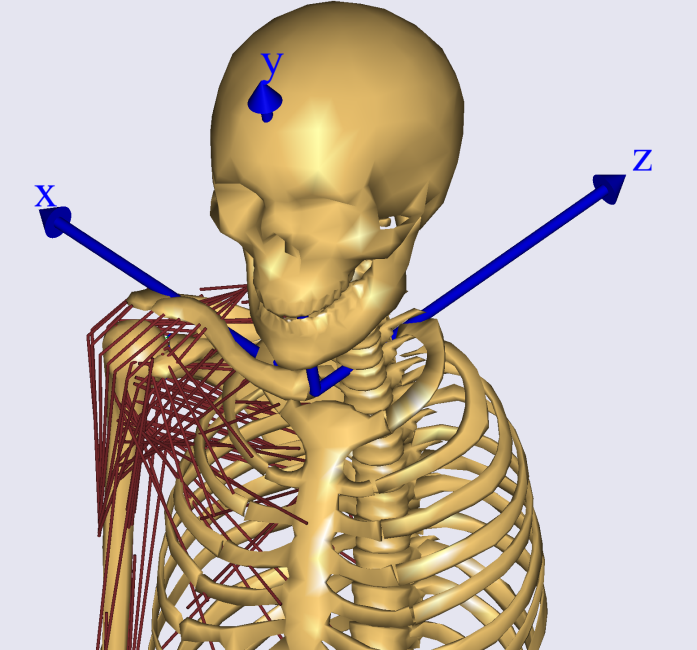
Next, we define the local ref frame on the clavicle. All forces will later be
exported with respect to this coordinate system. You can either use a
pre-defined reference system in the AMS or create a new one. The following lines
create a new node located in the Sternoclavicular joint. Insert it in the
Model\Environment.any file after the AnyFixedRefFrame GlobalRef:
  };
}; // END of GlobalRef

AnySeg &RiArm = Main.HumanModel.BodyModel.Right.ShoulderArm.Seg.Clavicula;
RiArm = {
  AnyRefNode localrefframe= {
      sRel = {0,0,0};
      // ARel = RotMat(0.5*pi,x);
      AnyDrawRefFrame drws = {ScaleXYZ = {1,1,1}*0.3;RGB={0,0,1};};
  };
};
Now, reloading the model should show the new reference frame in our model, where the left arm and all muscles, except those in the right arm, are switched off.
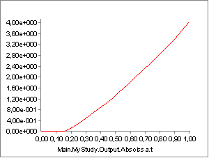
In this lesson, we want to make a FE analysis of the behavior of the clavicle
bone subjected to the applicable forces during a simple arm lift. First, change
the Mannequin.any file to create the desired physical activity. We want to
analyze a simple lifting case, so all we specify is flexion in the shoulder
joint. Open the Mannequin file and look for the PostureVel folder. Change the
Glenohumeral flexion value to 50/Main.Study.tEnd, this determines the joint
velocity necessary to reach 50-degree flexion taking into account the simulation
time.
Right = {
  //Arm
  SternoClavicularProtraction=0;   //This value is not used for initial position
  SternoClavicularElevation=0;    //This value is not used for initial position
  SternoClavicularAxialRotation=0; ///< Only used when the clavicular axial rotation rhythm is diabled

  GlenohumeralFlexion = 50/Main.Study.tEnd;
We also want to alter the initial starting position for the motion. In the
Posture folder also in the Mannequin.any file, make the changes indicated
below.
Right = {
  //Arm
  SternoClavicularProtraction=-23;   //This value is not used for initial position
  SternoClavicularElevation=11.5;    //This value is not used for initial position
  SternoClavicularAxialRotation=-20; ///< Only used when the clavicular axial rotation rhythm is diabled

  GlenohumeralFlexion =-0;
  GlenohumeralAbduction = 7;
  GlenohumeralExternalRotation = 0;

  ElbowFlexion = 5;
  ElbowPronation = -20.0;
We want this motion to be done in 10 seconds and analyze 5 time steps. This is
defined in the main file. In the Study folder, change the end time of the
study (tEnd) to 10 seconds and the number of time steps (nStep) to 5.
  AnyBodyStudy Study =
  {
    // Include the Model within the Study
    AnyFolder &Model = .Model;

    tEnd = 10.0;
    Gravity={0.0, -9.81, 0.0};
    nStep = 5;
Now download the prepared Abaqus file here,
which contains the mesh and geometry of the clavicle bone used in the model.
Save it in your working directory, meaning the folder where your main.any script
is located. Please note that this FE model of the clavicle was created in the
same reference frame as the clavicle model in the AnyBody model since we have
actually used the STL file exported from AMMR for this bone. Therefore,
localrefframe does not have to be displaced in order to match with the
coordinate system of the FE mesh. Had the FE mesh been generated based on
scanned data, the registration between AnyBody model’s clavicle and the FE mesh
can be entered using localrefframe’s sRel and Arel members.
In a similar manner, one could define a local reference frame in Abaqus by means
of the *SYSTEM keyword; however, this is not advisable because the AnyFE
Converter does not handle the *SYSTEM keyword in the supplied mesh file. We
shall return to the issue of aligning the coordinate systems for the AnyBody
forces and the mesh later, and so far we consider localrefframe to be aligned
with the mesh coordinate system.
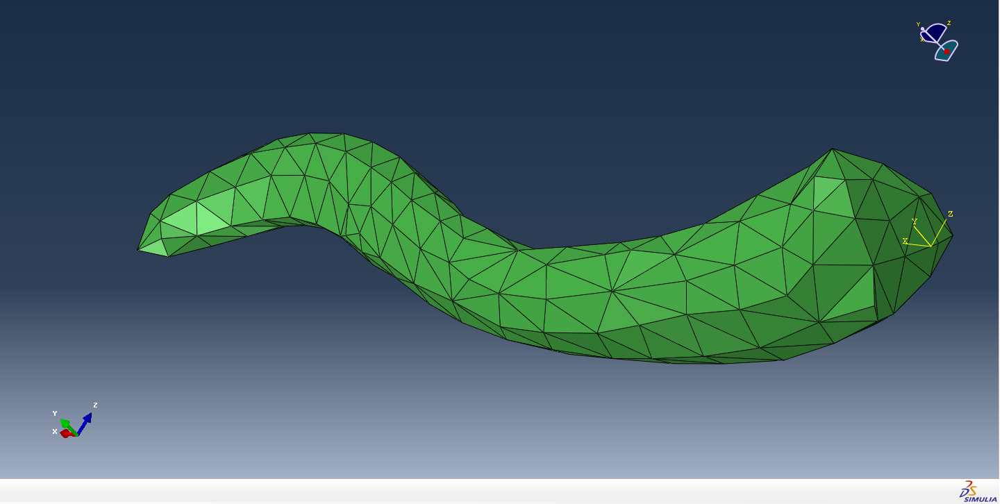
This figure below shows the clavicle bone mesh used for this tutorial. This bone is modeled with a reduced stiffness, which can be interpreted as an osteoporotic bone.
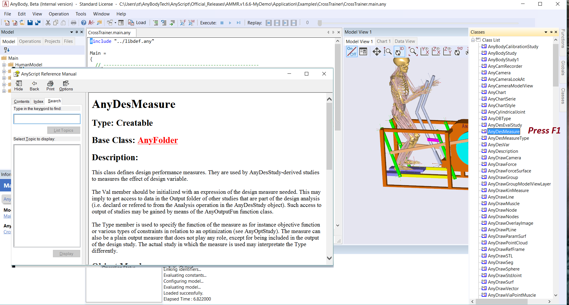
Exporting the Forces#
Now we have to specify which forces we want to export to the FE model. For this, we make use of the Class inserter tab. Place your cursor in the Study folder below the code shown above and select the ‘Classes’ tab on the right side of the AnyBody window. Under the folder ‘Class List’ search for the class named “AnyMechOutputFileForceExport” and double-click on it to insert the class necessary for exporting forces.
AnyMechOutputFileForceExport <ObjectName> =
{
  FileName = "";
  /*NumberFormat =
  {
  Digits = 15;
  Width = 23;
  Style = ScientificNumber;
  FormatStr = "";
  };*/
  //UseRefFrameOnOff = Off;
  //AllSegmentsInStudyOnOff = Off;
  //XMLformatOnOff = Off;
  //RefFrame = Null;
  //Segments = ;
  //MeshRefFrames = ;
  //ForceObjectExclude = ;
  //ForceObjectList = ;
  //AnyRefFrame &<Insert name0> = <Insert object reference (or full object definition)>;
  //AnyRefFrame &<Insert name1> = <Insert object reference (or full object definition)>; You can make any number of AnyRefFrame objects!
  //AnySeg &<Insert name0> = <Insert object reference (or full object definition)>;
  //AnySeg &<Insert name1> = <Insert object reference (or full object definition)>; You can make any number of AnySeg objects!
};
Create two new folders in your Human Standing model folder (the folder
containing the main.any script, the Model folder, and so on) named files_in
and files_out. This will be used to store the FE files. Now change the
inserted FE_out object as shown below. These definitions specify that all
forces acting on the segment Clavicula will be written in the xml file
“clavload.xml” and placed in the folder ‘files_in’. It is important to use the
xml format since the AnyFE converter only reads this format.
AnyMechOutputFileForceExport FE_out =
{
  FileName = "files_in/clavload.xml";
  UseRefFrameOnOff = On;
  RefFrame = &Main.HumanModel.BodyModel.Right.ShoulderArm.Seg.Clavicula.localrefframe;
  AllSegmentsInStudyOnOff = Off;
  XMLformatOnOff = On;
  Segments = {&Main.HumanModel.BodyModel.Right.ShoulderArm.Seg.Clavicula};
  MeshRefFrames = {&Main.HumanModel.BodyModel.Right.ShoulderArm.Seg.Clavicula.localrefframe};
};
The UseRefFrameOnOff option enables the specification of a reference frame in
which all forces and positions are reported. This is set to on and the
reference frame is specified to be the one we created before. The
AllSegmentsInStudyOnOff option is set to off, meaning not all segments in
the study are included, and the Segments option then specifies to only include
the clavicula segment.
This object will now write all the muscle and joint forces for all time steps in one xml file.
We are now ready to execute the AnyFE converter and transform the generic AnyFE XML file to an Abaqus readable INP file. Download the “AnyFE converter tool for Abaqus” at the AnyBody Technology webpage and unpack the files in your working directory folder, meaning the folder where your main.any script is located. These files include the AnyFE converter, which is an executable called “AnyFE2Abq.exe”. It can convert the xml code to Abaqus keyword sequence and combine it with the FE model.
For the AnyFE converter to work, you need to place your AnyBody license file in the same folder as the executable “AnyFE2Abq.exe”. To find your license file, click ‘Help’ in the top menu of your AnyBody window. Then click ‘Registration…’ and ‘View license status’. A window will open where the location of your license file is shown under the heading ‘License file(s):’. Go to the file location and copy your license file to the folder where the AnyFE converter is located. (IMPORTANT: do not delete the original license file when copying it)
The AnyFE converter is a command line tool with options controlled by program
arguments. You call the converter either from a shell prompt or from inside the
AnyBody system. The latter can be done by inserting the following code, where
the class AnyOperationShellExec is used. The names for the executable, its
working directory, and the options for the call of the executable file have to
be given. If you closely followed the tutorial, the paths in Arguments should
be correct, but please make sure the paths correspond to your setup, and then
insert the code below your study folder in the main file:
}; // END of Study

AnyOperationShellExec ConvertToAbq={
  Show=On;
  FileName = "AnyFE2Abq.exe";
  Arguments = "-i .\files_in\clavload.xml -o .\files_out\output.inp -m .\clavicula.inp";
  WorkDir=".\ ";
};
This will enter the operation called ConvertToAbq into the model and running
this will execute the AnyFE converter, where the file ‘clavload.xml’ is the
input, the file ‘output.inp’ is the output file and the file ‘clavicula.inp’ is
included in the output file.
We shall now briefly go through the important options for Arguments for the
AnyFE converter. The –i option specifies the input AnyFE xml file, which is
the file generated by the class AnyMechOutputFileForceExport, and the -o
option specifies the output file, which is the files to import in the Abaqus
model. The –m option is used to specify a FE model without boundary
conditions, which will be included in the output file by means of an
include-statement. In this case, the downloaded Abaqus INP-file
(“clavicula.inp”), containing only the mesh, will be included in the converter
output (“output.inp”), also an INP-file.
Another significant option is –e, which is the radius of muscle/ligament
attachment area. This radius (default value is 1 cm) is used for the
construction of coupling constraint between a loaded point and the surface of
the bone. Please note that this radius is used on all loads applied, not only
muscles and ligaments, but also joint reactions, applied loads, etc. This
parameter is not a physiological parameter. Please also note that in case of
complex concave geometries these constraints may select wrong parts of the bone
surface and may require some manual adjustments.
For more information on the used classes AnyMechOutputFileForceExport and
AnyOperationShellExec, go to the AnyScript Reference Manual and search for the
two names.
👉 Now you are ready to run the analysis and convert the data. Reload the
Anybody model and run the operation ‘RunApplication’. This will automatically
run the ‘Calibration’ and ‘InverseDynamics’ studies. Next, run the
‘ConvertToAbq’ operation. This will create a new Abaqus input file in the
files_out folder called “output.inp”.
Using the Shell Prompt and More Details on the AnyFE Converter#
You can achieve the same result using the shell prompt by executing the following command:
AnyFE2Abq.exe -i ..\files_in\clavload.xml -o ..\files_out\output.inp -m .\clavicula.inp
At this point, let us return to the issue of the coordinate systems that we have
used so far and an alternative option. In the example, we have exported all the
positions and forces with reference to a given manually defined system attached
to the clavicle, i.e. the ‘localrefframe’. The AnyFE converter will by default
transfer all positions and forces directly, i.e., in the same coordinate system
as exported the AnyFE XML file. In the above, we have therefore considered
‘localrefframe’ to be the coordinate system of the FE model, which is also the
CT/MRI scan system. Notice that in the given case, the segment reference and the
output reference are aligned since the FE mesh was based on the original bone
geometry from the AnyBody model, i.e. sRel= {0, 0, 0}.
As an alternative, you can export the AnyFE XML file in another reference frame,
even the global system in AnyBody (UseRefFrameOnOff=Off) for that matter. This
implies that the data of the AnyFE XML file may or may not contain motion of the
bone and it will probably not be aligned with the FE mesh/CT/MRI scan system. If
you chose this option, the AnyFE Converter can remove the rigid body motion by
using the –r option equal to ‘segment’:
AnyFE2Abq.exe -i ..\files_in\clavload.xml -o ..\files_out\output.inp -m .\clavicula.inp –r segment
This makes all AnyFE data from the AnyFE Converter being transformed to the local frame of the segment, here the clavicle segment, before applied to the FE model and outputted.
If the reference frame of the segment is not identical to the one of the FE
mesh, one can apply a constant transformation to all data accommodating for this
misalignment. The –t option allows you to enter the transformation as a string
containing space-separated numbers. The command line will look like:
AnyFE2Abq.exe -i ..\files_in\clavload.xml -o ..\files_out\output.inp -m .\clavicula.inp –r segment –t "a11 a12 a13 a21 a22 a23 a31 a32 a33 dx dy dz"
The transformation may contain either 9 or 12 numbers. The first nine, aij, must be the orthogonal rotational transformation matrix and the latter optional three, dx, dy, and dz, are the translations.
These options allow you to handle the coordinate systems differences using the AnyFE Converter, i.e., outside AnyBody. For instance, this implies that you do not have to redo simulations just to apply the same forces to another FE mesh with another local frame; this can all be done with adjustment of the parameters for the AnyFE converter.
However, in this tutorial, we will not use these options to specify another
reference frame, so you do not need to include the –r and –t options. Now
that we have looked at how to execute the AnyFE converter properly, let’s have a
closer look at what it does.
Please notice that the AnyFE Converter is reading the Abaqus input file (INP)
and it is only expecting a simple mesh specification. This reader is not fully
compatible with the INP keyword language for Abaqus. Basically, it only reads in
the first block of nodes (*NODE section) and it does not accept commands that
may interfere with the interpretation of this node section. This implies that
many Abaqus keywords are not allowed in front of the first node section. This
also implies that subsequent node sections are not read and therefore, not used
for application of forces.
When the AnyFE Converter is executed, it performs the following actions:
Maps all AnyBody exported forces, i.e., joint reactions, muscle forces and applied forces to the provided FE mesh. Mass related forces are neglected, i.e., gravitational and acceleration equivalent forces.
Defines nodes in the positions from the AnyFE output file, i.e. the position of all loads (this includes muscle/ligament attachment nodes)
Defines amplitudes for each force/moment component in the AnyFE output file
Defines concentrated loads (
*CLOAD) in each of these nodesDefines coupling constraints between the created nodes and a part of the surface of the bone
Includes the mesh
Adds inertia relief loads (
*INERTIA RELIEF)
Please note that the inertia relief loads will automatically be added to the model in order to provide a full set of boundary conditions. However, these loads require a density value in the material definition section (which already is defined in the downloaded ‘clavicula.inp’ file). Absence of this density value will result in an error during the FE analysis. In case when additional constraints are present in the model, e.g. environment support, contact with another bone, etc., the inertia loads can be suppressed or removed.
Importing and Modifying the Model in Abaqus#
Open Abaqus and import the input file from the files_out folder as a Model.
This will load the clavicula mesh model and apply the boundary conditions
exported from the AnyBody Model. The Abaqus model is now ready to run the finite
element analysis directly and then post-process the results. You can also make
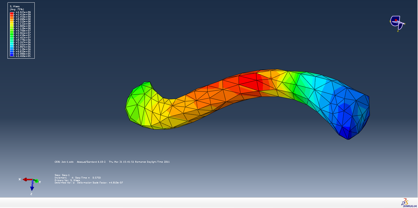
custom adjustments to the model before running. The image below shows the
results of running the model without any custom adjustments, where the von Mises
stress plot can be seen.
Tip
Instructions on how to load the model and run Abaqus analysis:
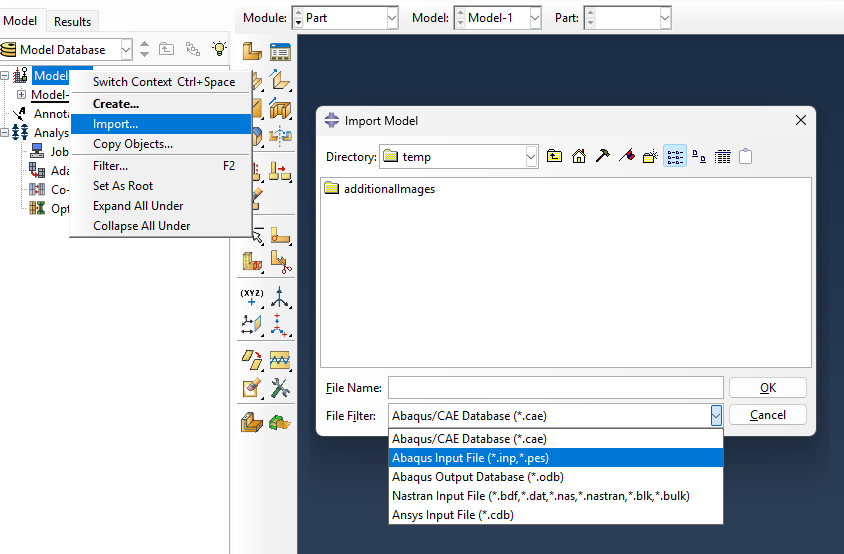
Right-click on ‘Models’ and select ‘Import…’
In the pop-up dialog selected file extension to be ‘.inp’
Select INP file generated in this tutorial and click ‘OK’
Right-click on ‘Jobs’ and Create new job.
Select your loaded model called ‘output’, name the job and click ‘Continue…’
In the pop-up window, you can edit your job - for this tutorial, we don’t change any settings, so click ‘OK’
Expand the Jobs folder to see your newly created job. Right-click on the job and select ‘Submit’.
When the job is completed you can view the results by right-clicking on the job and selecting ‘Results’.
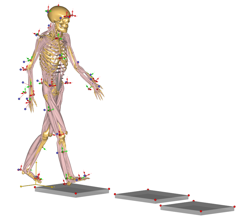
In the following picture, you can see the muscle attachments nodes and coupling constraints that are applied to the finite element model. These are found under the ‘Constraints’ folder in Abaqus. Each group of yellow lines defines one muscle attachment by a point and a surface area on the model to attach, and corresponds to a similar muscle attachment in the AnyBody model.
Note
By comparing the muscle attachment in the Abaqus model with the muscle attachment in the AnyBody model, you can see that the sternocleidomastoid muscle attachment is missing in the Abaqus model. This is because the AnyFE Converter excludes all muscles that carry zero load, when generating the Abaqus input file.
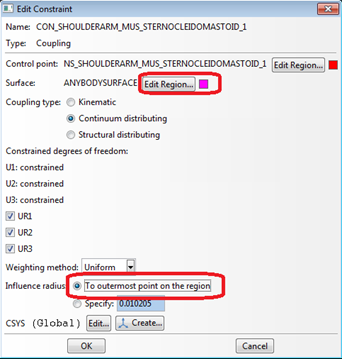
Bear in mind that the muscle attachment area is considered to have a constant radius, however, in reality, these areas are often elongated and have an irregular pattern. To better fit the user’s expectations, for example, to be more physiological, each constraint can be modified. That can be done by defining the desired muscle attachment area as a new surface in the Abaqus model and changing the relevant coupling constraint to refer to this surface. When doing this, it is important to set the influence radius option to ‘To outermost point of the region’ when editing the constraint, to make sure that all points on the specified surface area are included in the constraint.
This completes Lesson 3 and hereby the lessons on the interfacing between the
AnyBody Modeling System and Finite Element systems. The final AnyBody script and
Abaqus model can be downloaded here.
Please remember to place your downloaded AnyFE2Abq.exe and your license file in
the same folder, before running the AnyFE converter.
For more information on how to build and design a CAD model, which can be imported into AnyBody to interact with a human model, see the following tutorial: Making Models using SOLIDWORKS.