Lesson 1: The Basics of Muscle Recruitment

Old tutorial:

This tutorial has not yet been updated to ver. 7 of the AnyBody Modeling System. Some concepts may have changed.

Muscle recruitment in inverse dynamics is the process of determining which set of muscle forces will balance a given external load. If we take the trouble of setting up the system of equilibrium equations for a musculoskeletal system by hand, then we can organize them on the following form:

\[ \mathbf{Cf}=\mathbf{r} \]

where f is a vector of muscle and joint forces, r is a vector representing the external forces and inertia forces, and C is a matrix of equation coefficients. In other words, equilibrium always results in a linear system of equations that should be easy to solve. Unfortunately, it is not, and this is due to two reasons.

The first reason is that muscles are unilateral element that can only pull and not push. So the part of f that is muscle forces is restricted in sign, and only solutions with positive or zero muscle forces are physiologically reasonable.

The second reason is known as muscle redundancy. It is due to the fact that muscle systems tend to have many more muscles than strictly necessary to balance the external forces. The mathematical consequence is that the equilibrium equation above has more unknowns than it has equations and therefore usually infinitely many solutions.

So, is muscle recruitment in the living human body random in the sense that it just chooses the first and the best solution that balances the load? Experiments show that this is not the case. In skilled movements, muscles tend to be recruited systematically, so there is some criterion behind the central nervous system’s choice of muscle activations. Mathematically we can formulate the choice between the infinitely many solutions as an optimization problem in the following way:

\[\begin{split} \begin{equation*} \begin{aligned} & {\text{minimize}} & & G\left(\mathbf{f^{(M)}}\right) \\ & \text{subject to} & & \mathbf{Cf} = \mathbf{r} \\ &&& f_i^{(M)} \geq 0, i=1\ldots n^{(M)} \end{aligned} \end{equation*} \end{split}\]

The equilibrium equations are constraints in this problem: whatever solution we find must balance the external forces. The requirement for positive muscle forces has also been added as a constraint to the problem. Only solutions adhering to these two requirements are acceptable, but out of these many solutions we are going to change the one that minimizes the function G, and are furthermore going to anticipate that this function depends on the muscle forces. This seems reasonable because muscle recruitment is probably a result of biological adaptation and muscle work is costly for the organism and should be minimized in an environment where resources are limited. Now we just have to figure out what the function G actually is and unfortunately there is nobody around who knows it for sure.

So in the following we are going to play around with different choices and see what happens. AnyBody is great for this purpose because the settings of the InverseDynamics operation offer the user a lot of freedom to choose the function he or she believes is the right one for a given purpose.

So let’s get set up with a model that is suitable for experimentation with different definitions of the muscle recruitment problem. We shall begin with one that is very, very simple and work our way upwards from there. Please download right-click this link and save the file in a working area of your hard disk: Recruitment.Main.any.

Open the model in the AnyBody Modeling System, load it into memory, open a Model View window, select the InverseDynamics operation, and click the Run button. You should see something like this:

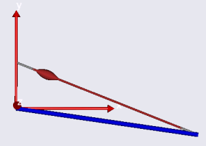
The thick blue rod is an arm hinged at its left end to the origin of the global reference frame. A muscle is attached at the other end and the muscle elevates the arm against gravity.

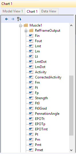
Please click Window->Chart (2D) to open up a new window for inspection of results. You can expand the tree on the left hand side of that window and find the muscle force, Fm, somewhere inside the properties of the M1 muscle. When you click it you get a graphical representation of the muscle force:

Obviously, AnyBody has solved the equilibrium equations and has determined what the muscle force is at every instant of the simulation time. But which objective function, \(G\), has the system used?

If we review this problem we can see that it has only a single degree of freedom and only a single muscle to carry the load. This actually means that the equilibrium equations are determinate (one degree of freedom and one muscle) and in this case it does no matter what \(G\) is, so there is little we can do in the settings to influence the result of the analysis. The result is given by equilibrium alone and there is no other muscle force than the one you see in the graph that would be able to balance the model. It does not get really interesting until we apply another muscle. A couple of simple additions to the model will accomplish this. We first add a new origin node on the global reference frame:

Main = {
  // The actual body model goes in this folder
  AnyFolder MyModel = {
    // Global Reference Frame
    AnyFixedRefFrame GlobalRef = {
      AnyDrawRefFrame drw = {
        ScaleXYZ = {1,1,1}/10;
        RGB = {1,0,0};
      };
      AnyRefNode M1 = {
        sRel = {0, 0.05, 0};
      };
      AnyRefNode M2 = {
        sRel = {0, 0.03, 0};
      };
    }; // Global reference frame

Then we define a second muscle by copying the first one and making a few changes. Notice that the strength of the second muscle is set to half of the strength of the first one:

AnyMuscleViaPoint M1 = {
  AnyMuscleModel Model = {
    F0 = 100;
  };
  AnyRefFrame &Ori = .GlobalRef.M1;
  AnyRefFrame &Ins = .Seg.M;
  AnyDrawMuscle drw = {
    Bulging = 1;
    MaxStress = 1e5;
  };
};
AnyMuscleViaPoint M2 = {
  AnyMuscleModel Model = {
    F0 = 50;
  };
  AnyRefFrame &Ori = .GlobalRef.M2;
  AnyRefFrame &Ins = .Seg.M;
  AnyDrawMuscle drw = {
    Bulging = 1;
    MaxStress = 1e5;
  };
}; 

Now two muscles will have to cooperate on the task of carrying one degree of freedom. Let us see what AnyBody, in the absence of any special specifications from the user, chooses to do. If you load and run the model, plot the muscle force of M1 as you did before, and then manually place an asterisk in place of the muscle name in the specification line in the Chart window, you should get something like this:

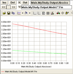
We can observe that both muscles are working and that M1, which has the higher strength and better moment arm, is exerting more force than the weaker M2. This seems immediately reasonable from a physiological point-of-view, and this is what you get from AnyBody if you do not make any special specifications. We shall get back to the precise nature of AnyBody’s standard criterion a little later. For now, let us proceed and speculate a bit about what may or may not make physiological sense in lesson 2.