
Lesson 1: Personalizing Individual Segments Based on Geometric Data from Medical Images#
Note
This tutorial presumes that you have read the AMMR documentation and know how to personalize your model using information about height, weight, and individual segment lengths.
In this lesson you will learn how to personalize a bone segment (the femur) so a generic model matches a specific person’s anatomy from medical imaging. We do this by scaling the bone surface, starting with basic affine transformations and advancing to more sophisticated nonlinear methods.
You will be introduced to an advanced approach to scaling based on a sequence of affine and non-affine transformations. Each of these transforms is constructed based either on subject-specific geometry or on a set of landmarks selected on the bone surface. As opposed to the simple scaling laws explained in the AMMR documentation, this lesson is rather methodological than conceptual and provides a good overview of how to pipeline and combine different 3D transforms to obtain subject-specific morphing and registration between frames of reference.
Shortly explained, the sections in this lesson are as follows:
Linear Point-Based Scaling: Using a set of matching landmarks (points) on the source and target geometries to construct a linear transform (move, rotate, scale, and skew) that scales the source into the target geometry.
Landmark-Based Nonlinearities: Refining the scaling by adding a nonlinear transform fitted to a new set of matching landmarks (points).
Surface-Based Nonlinearities: Further refining the scaling by adding a nonlinear transform fitted to the surfaces of the source and target geometries.
Linear Point-Based Scaling#
The simplest inclusion of the subject-specific bone shape from medical image data is to find the affine (linear) transformation that fits a number of corresponding points that are selected on the source and the target geometries. These points could be fitted e.g. in a least-squares manner. This approach is similar to utilizing external body measurements as it relies on a linear transform. However, it is less dependent on the bone orientation and prior knowledge of dimensions to be measured. For example, you can locate any two points on source and target surface consistently without thinking of how a segment length was measured.
Let us make a simple example of using landmark-based affine scaling.
First, please download two femur surfaces,
SourceFemur.stl and
TargetFemur.stl and save them in your
working directory. These femur geometries will be used for the rest of
this tutorial. The source surface is an unscaled femur used in the
standard AnyBody models in the AMMR. The target surface is a femur
reconstructed from a CT image and saved as a surface mesh in STL format
(courtesy of Prof. Sebastian Dendorfer, OTH Regensburg,
Germany).
Next, please download the AnyScript file
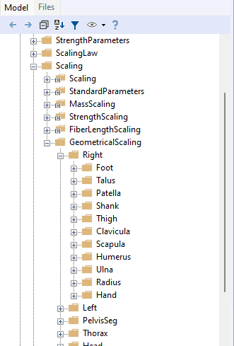
lesson1a.main.any. This file contains
a model with two segments which contain the definition of a surface
each, one for the source (bone color) and one for the target (yellow) bone. When we load this
model, the Model View should show the following picture:
To define a new scaling function let us insert a new AnyFunTransform3DLin2
object after the target segment:
  AnySeg TargetFemur = {
    Mass = 0; Jii = {0, 0, 0};
    AnyDrawSurf Surface = {
      FileName = "TargetFemur.stl";
      RGB = {256,256,0}/256;
    };
  };

  AnyFunTransform3DLin2 <ObjectName> = {
    //PreTransforms = {};
    Points0 = ;
    Points1 = ;
    //Mode = VTK_LANDMARK_RIGIDBODY;
  };

}; // MyModel
The AnyFunTransform3DLin2 object allows us to build a transform that
fits a set of source and target landmarks in a least-squares manner.
The object constructs a linear transforms in a full
affine (linear transformation with translation, rotation, size-scaling
and skewing, i.e. 12 degrees of freedom), uniform (orthogonal rotation
with uniform scaling and translation, i.e., 9 d.o.f.), or rigid-body
manner (orthogonal rotation of unscaled object with translation, i.e., 6
d.o.f.). Please note that the AnyFunTransform3DLin2 object utilizes the
vtk-function/filter vtkLandmarkTransform, and, therefore inherits its
modes:
VTK_LANDMARK_AFFINEVTK_LANDMARK_SIMILARITYVTK_LANDMARK_RIGIDBODY
A description of this function can be found here.
For this example we want to register our source surface into the target one by using a
full affine transform. Therefore, we select several corresponding points
on the surfaces and put them into the two point-sets called “Points0” and
“Points1”, which are the source and target points, respectively. As the next
step, we change the mode of the AnyFunTransform3DLin2 object to
VTK_LANDMARK_AFFINE to use the affine transform:
AnyFunTransform3DLin2 MyTransform = {
  //PreTransforms = {};
  Points0 = {
    {-0.00906139,    0.36453,  0.0175591}, // fovea capitis
    {0.0358368,   -0.0100391, -0.0162062}, // lateral anterior condyle
    {0.0295267,   -0.0112881,  0.0194889}, // medial anterior condyle
    {0.0282045,     0.157599, -0.0172379}, // anterior mid shaft
    {-0.0245689, -0.00701566, -0.0238393}, // lateral posterior condyle
    {-0.0320739, -0.00877602,  0.0244234}  // medial posterior condyle
  };

  Points1 = {
    {0.289913,0.420538,0.0138931},     // fovea capitis
    {0.322038,0.433232,-0.378636},    // lateral anterior condyle
    {0.289309,0.426839,-0.372994},    // medial anterior condyle
    {0.328859,0.425856,-0.175012},    // anterior mid shaft
    {0.306293,0.487243,-0.370319},    // lateral posterior condyle
    {0.261891,0.47585,-0.372696}      // medial posterior condyle
  };

  Mode = VTK_LANDMARK_AFFINE;
};
Tip for landmark selection
If you want to extract the coordinates of the points on the surfaces in your own
model, you can use the open source software MeshLab, which can be downloaded
here.
Import the STL surface into MeshLab
Use the
PickPointstool to select points on the surface by right-clicking on the desired locations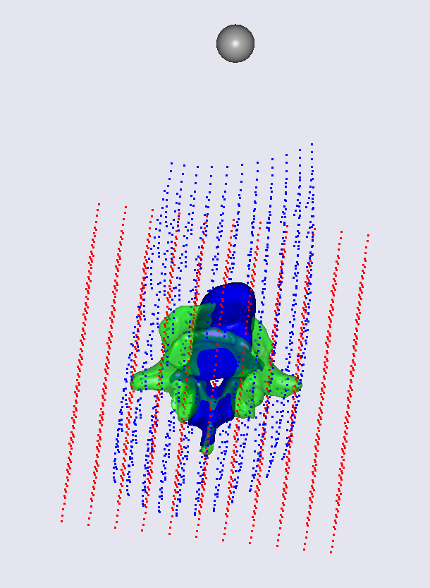
Save the points to a file
Open the saved file in a text editor and copy the coordinates of the points into your AnyScript model (be aware of the order of the x-, y-, and z-coordinates)
The selected points on the surface represent specific anatomical landmarks and points described in the comments of the AnyScript code. Final modification before we can use the constructed linear transform is to give this transformation a name and apply it to the source surface:
AnySeg SourceFemur = {
  Mass = 0; Jii = {0, 0, 0};
  AnyDrawSurf Surface = {
    FileName = "SourceFemur.stl";
    RGB = {222,202,176}/256;
    AnyFunTransform3D &ref = ..MyTransform;
  };
};
Reloading the model and looking at the bones shown in the Model View, we can see that these bones are now merged. It will produce the following picture.

The source bone is now transformed, i.e., translated, scaled and
skewed to match the target bone. To clearly view the difference between
the transformed and the original source surface, let us add a new
AnyFunTransform3DLin2 called “MyTransform2” to the model that we place
after “MyTransform”. The intention is to construct a reverse rigid-body
registration transform between target and source surface. Please note,
the roles of the source points “Points0” and target points “Points1” are swapped,
and the transformation mode is set to VTK_LANDMARK_RIGIDBODY.
Additionally to that, a combination transform, containing the forward affine and back registration transforms, is added and named “MyTransform3”:
};  //End of MyTransform

AnyFunTransform3DLin2 MyTransform2 = {
  Points0 = .MyTransform.Points1;
  Points1 = .MyTransform.Points0;
  Mode = VTK_LANDMARK_RIGIDBODY;
};

AnyFunTransform3DIdentity MyTransform3 = {
  PreTransforms = {&.MyTransform,&.MyTransform2};
};
Finally, let us look at the effect of the constructed transform. We comment the transform used in the visualization of the source surface and create another surface that will show the combined transformation that we just constructed:
AnySeg SourceFemur = {
  Mass = 0; Jii = {0, 0, 0};
  AnyDrawSurf Surface = {
    FileName = "SourceFemur.stl";
    RGB = {222,202,176}/256;
    // AnyFunTransform3D &ref = ..MyTransform;
  };

  AnyDrawSurf SurfaceMorphed = {
    FileName = "SourceFemur.stl";
    AnyFunTransform3D &ref = ..MyTransform3;
  };
};
Looking at the Model View, we can see that the femur is now scaled. It became longer and now aligns with the original source femur position. From the previous picture, we also know that geometry is matching the target quite well too (and if you want to convince yourself, you can superimpose the target geometry using the “MyTransform2” reverse registration transformation in the visualization of the target surface).
With this example, we have shown how to morph the source into the target with a full affine scaling and subsequently applying a reverse registration to move the morphed geometry back.
Notice that it is possible to reverse the combination, i.e., to apply the registration step first and then the scaling/morphing step. For instance, make a transformation similar to “MyTransform”, but insert “MyTransform2” as pre-transformation. In this tutorial lesson, we shall however stay with the concept we presented so far.
If the morphing accuracy is sufficient for your task you can proceed with your modeling and stop at this step. However, for the purpose of this tutorial, the desired accuracy has not been reached - some local features still do not match the target features, e.g. the lesser and the greater trochanter. The following steps explain how to capture more details and improve morphing for even better match.
Incorporating Landmark-Based Nonlinearities into the Scaling Function#
The next level of detail can be achieved by introducing local nonlinear deformations
by means of the AnyFunTransform3DRBF class. This class represents a nonlinear
interpolation/extrapolation transformation, which is based on the Radial Basis Functions (RBF)
method and uses landmarks selected on source and target surfaces. Detailed behaviour
of this transform is described in an appendix tutorial.
However, the focus of this tutorial is to demonstrate available pipelines of transforms. For
simplicity, we use a preselected set of femoral landmarks and RBF settings.
We start with the model from the previous steps to introduce the landmark-based
nonlinear scaling. Several tranformations will build up into a pipeline, where
pre-transforms will be used to inherit obtained accuracy throughout different steps.
You can find the complete model here: lesson1b.Main.any.
The following tutorial shows how to add an RBF transform with the recommended settings
into the previously created model.
First of all, let us configure the visualization of the transformation. Now that we know how to compare source and scaled geometries as well as reverse registration, we can switch off the registration step.
AnyFunTransform3DIdentity MyTransform3 = {
  PreTransforms = {&.MyTransform/*,&.MyTransform2*/};
};
This will return our morphed geometry back to the target bone location and we
can observe the improvements as we go. Let us now define an RBF transformation,
AnyFunTransform3DRBF, and another AnyDrawSurf object that will show the
difference between the affine scaling and the new transformation pipeline
employing nonlinear RBF transformations, both placed on top of the target
bone. For a better contrast of the different surfaces, we will also add some
colors to the drawing of the surfaces.
First, insert the following code below “MyTransform3” to define the new RBF transformation:
AnyFunTransform3DRBF MyRBFTransform = {
PreTransforms = {&.MyTransform};
PolynomDegree = 1;
RBFDef.Type = RBF_Triharmonic;
Points0 = {
{-0.00920594, 0.36459700, 0.0174376}, // fovea capitis
{ 0.03691960, -0.01011610, -0.0197803}, // anterior lateral condyle
{ 0.03001110, -0.00998133, 0.0186877}, // anterior medial condyle
{ 0.02009270, 0.34511400, -0.0387426}, // anterior greater trochanter point
{ 0.02783850, 0.18320400, -0.0217463}, // anterior shaft point
{-0.02461770, -0.00623515, -0.0231383}, // posterior lateral condyle
{-0.03211040, -0.00908290, 0.0246153}, // posterior medial condyle
{-0.02643670, 0.35630800, 0.0014140}, // posterior head point
{ 0.01780310, 0.36194400, 0.0059740}, // anterior head point
{-0.00197744, 0.38387300, -0.0031698}, // superior head point
{-0.00316772, 0.34248600, 0.0114698}, // inferior head point
{-0.02469710, 0.30335600, -0.0171113}, // medial lesser trochanter
{-0.00969883, 0.34826800, -0.0462823}, // distal trochanteric fossa
{-0.01959660, 0.36243100, -0.0441186}, // proximal posterior greater trochanter
{-0.00084335, 0.32253400, -0.0641596}, // distal trochanteric fossa
{-0.00431680, 0.35912600, 0.0036940} // femoral COR
};
PointNames = {
"Medial_Head_Point",
"Anterior_LateralCondyle_Point",
"Anterior_MedialCondyle_Point",
"Anterior_GreaterTrochanter_Point",
"Anterior_Shaft_Point",
"Posterior_LateralCondyle_Point",
"Posterior_MedialCondyle_Point",
"Posterior_Head_Point",
"Anterior_Head_Point",
"Proximal_Head_Point",
"Infeior_Head_Point",
"Medial_LesserTrochanter_Point",
"Distal_TrochantericFossa_Point",
"Proximal_Posterior_GreaterTrochanter_Point",
"Lateral_Lesser_Trochanter_Point",
"Femoral_COR"
};
Points1 = {
{ 0.2900, 0.4205, 0.0139},
{ 0.3220, 0.4332,-0.3786},
{ 0.2893, 0.4268,-0.3730},
{ 0.3599, 0.4429,-0.0050},
{ 0.3289, 0.4259,-0.1750},
{ 0.3062, 0.4872,-0.3703},
{ 0.2619, 0.4759,-0.3727},
{ 0.2900, 0.4405, 0.0139},
{ 0.3200, 0.4095, 0.0134},
{ 0.3100, 0.4295, 0.0314},
{ 0.2983, 0.4196,-0.0066},
{ 0.3089, 0.4599,-0.0355},
{ 0.3349, 0.4579, 0.0050},
{ 0.3329, 0.4679, 0.0175},
{ 0.3519, 0.4599,-0.0355},
{ 0.3075, 0.4235, 0.0139}
};
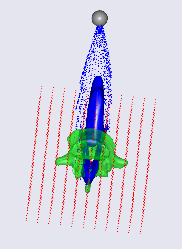
BoundingBox = {
Type = BB_Cartesian;
ScaleXYZ = {2, 2, 2};
DivisionFactorXYZ = 5*{1, 1, 1};
};
BoundingBoxOnOff = On;
};
}; // MyModel
To visualize the effect of this transformation, now add a new AnyDrawSurf object
in the “SourceFemur” segment.
  AnyDrawSurf SurfaceMorphed = {
    FileName = "SourceFemur.stl";
    AnyFunTransform3D &ref = ..MyTransform3;
  };

  AnyDrawSurf SurfaceMorphedRBF = {
    FileName = "SourceFemur.stl";
    AnyFunTransform3D &ref = ..MyRBFTransform;
    RGB={1,0,0};
  };
}; // AnySeg SourceFemur
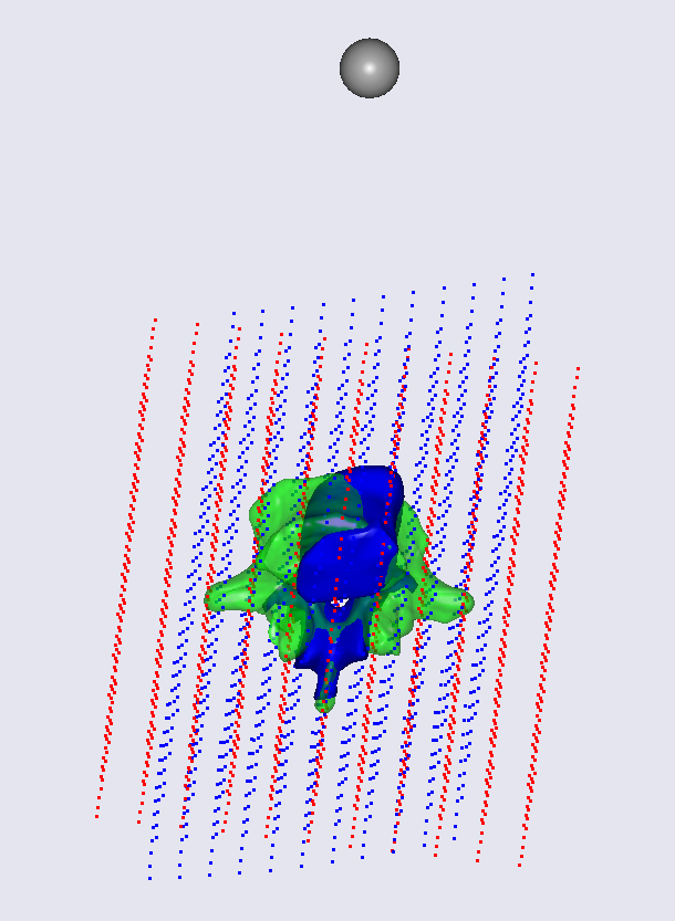
Loading the model, should now show the target bone (yellow), the affine scaled bone (grey), and the RBF-scaled bone (red) on top of each other, as shown in the figure below:
This code constructs a transform, which deforms the source geometry
into the target geometry using the thin-plate interpolation method and minimizes
the distance between the selected key points (landmarks). This can be used
when certain muscle attachment areas/points need to be scaled. Using this
allows us improving the model by making some local features more accurate
for the sensitive analyses. Please note that MyTransform object was
included as a pre-transform as a rough scaling preceding the nonlinear
RBF function, and it will be applied to the source entities, i.e. achieving
the result of the previous step.
Tip
Placing your mouse over objects in the Model View shows the name of the object.
However, it is still possible to improve the fitting of the femur surfaces and, thus, improve the accuracy of the model. Looking at the Model View you can notice that the red and yellow surfaces are slightly different, e.g. at the femoral head region. This is caused by the nature of the interpolation and a low number of control points. The following section will describe how to utilize surface information for the construction of an improved scaling law.
Incorporating Surface-Based Nonlinearities into the Scaling Function#
In this section, next improvement to the morphing is added by utilizing
surface information. The surfaces will be requested to be morphed into each
other, which will at the same time deform all related soft tissue attachment
points accordingly. The AnyFunTransform3DSTL class is used for this purpose.
This class constructs an RBF transformation similarly to the AnyFunTransform3DRBF
by using either 1) corresponding vertices on the STL surfaces or 2) seeding a number
of vertices on one surface and finding a matching closest point on the second.
Note
For constructing a transformation using the vertices of STL surfaces, the surfaces have to be topologically equivalent, i.e. the surfaces have the same number of triangles and each neighbor and vertices represent the same features on both surfaces.
For the latter option, we require an acceptable pre-registration transform, e.g. the RBF transform that was described previously, in order for the closest point search to make sense. Due to the implementation specifics, most of the RBF recommendations apply to this class as well. More details about how to create this kind of transforms are described in the appendix to this tutorial. However, for this example, the recommended settings mentioned before will be used again.
You can download the model with all modifications so far
here.
Now let us repeat the step from the previous section first by defining the new
scaling transformation using AnyFunTransform3DSTL and naming it “MySTLTransform”:
  }; // End of MyRBFTransform

  AnyFunTransform3DSTL MySTLTransform = {
    PreTransforms = {&.MyRBFTransform};
    PolynomDegree = 1;
    RBFDef.Type = RBF_Triharmonic;
    AnyFixedRefFrame Input = {
      AnySurfSTL SourceSurf = {
        FileName = "SourceFemur.stl";
        ScaleXYZ = {1, 1, 1};
      };
      AnySurfSTL TargetSurf = {
        FileName = "TargetFemur.stl";
        ScaleXYZ = {1, 1, 1};
      };
    };

    SurfaceObjects0 = {&Input.SourceSurf};
    SurfaceObjects1 = {&Input.TargetSurf};
    //FileName0 = "SourceFemur.stl";    // such definition was used previously
    //FileName1 = "TargetFemur.stl";    // such definition was used previously
    NumPoints = 1000;
    BoundingBox.ScaleXYZ = {2, 2, 2};
    BoundingBox.DivisionFactorXYZ = {1, 1, 1};
    BoundingBoxOnOff = On;
  };
}; // MyModel
Then we add a new AnyDrawSurf object to visualize the surface of this new
transformation:
  AnyDrawSurf SurfaceMorphedRBF = {
    FileName = "SourceFemur.stl";
    AnyFunTransform3D &ref = ..MyRBFTransform;
    RGB={1,0,0};
  };

  AnyDrawSurf SurfaceMorphedSTL = {
    FileName = "SourceFemur.stl";
    AnyFunTransform3D &ref = ..MySTLTransform;
    RGB={0,0,1};
  };
}; // AnySeg SourceFemur
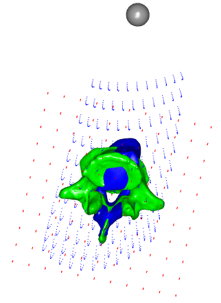
Please note again the transform from the previous section of this tutorial was included as a pre-transform, which means we will start working with the result of the previous step. Reloading the model, we can now see all steps of scaling in one place and can switch them on and off. For example, let us try to hide affine and RBF scaled femurs to see the final results:
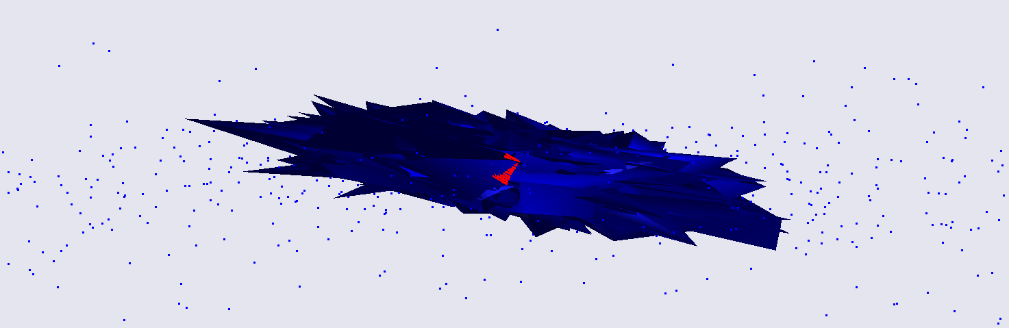
If we just look at the yellow target surface and the blue STL-transformed
surface, we can see that the surfaces now match each other very well. That means
that now the subject-specificity will be taken into account in the inverse
dynamics simulation. The final model can be downloaded
here.
Finally, the only thing left is to include this scaling function into an actual model. Lesson 2 describes how this can be done.