Lesson 4: Using Surfaces to Define the Knee Joint

The knee model developed in the previous lessons is obviously very simple and does not resemble the geometry of a real anatomical knee very well. However, AnyBody also contains facilities for development of more realistic geometries of surfaces such as the femoral condyles, and we shall explore those in this lesson. We start from the model developed in the third lesson. If you did not manage to obtain a working model from the third lesson, then please download a new one here.

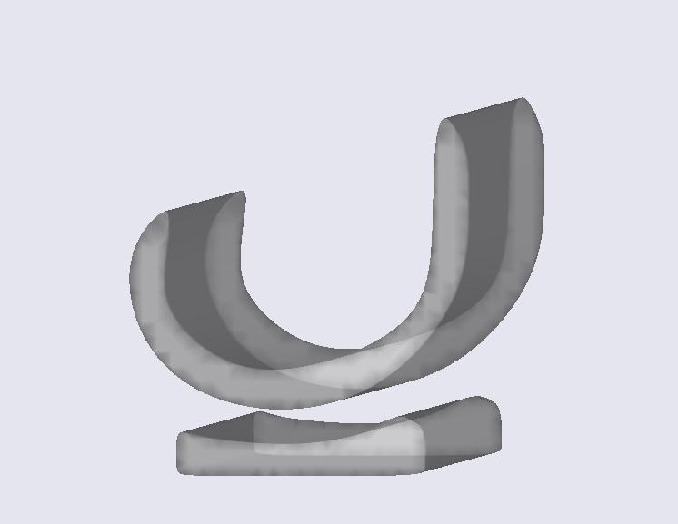
In this example, we are modeling the knee joint using some simplified 2-D implants (see picture) for the femoral head and the tibial plateau. To do this, we add some STL surfaces for theses implants to the model and use them to calculate a contact force, which changes the joint kinematics by making the implant surfaces slide along each other in the simulated motion.

Warning

Please note that if the surface has thin parts is a good idea to remove the backside of the surface so that it becomes open. This ensures that the forces will continue to grow as the surfaces are compressed into each other.

Due to the Force Dependent Kinematics (FDK), the joint axis for the knee moves as a function of external forces and muscle forces. In this lesson we want to have a closer look at this migration. Before inserting the implant, we relocate the position of the insertion node of the quadriceps muscle on the tibia back to the initial position.

AnySeg Shank = {
  r0 = {0.8, -0.4, 0.0};
  Mass = 4;
  Jii = {0.4, 0.01, 0.4}*0.4;
  AnyDrawSeg drw ={
    Opacity = 0.5;
    RGB = {1,0,0};
  };
  
  AnyRefNode KneeCenter = {
    sRel = {0.0, 0.4, 0.0};
  };
  AnyRefNode Quadriceps = {
    sRel={0.05, 0.3, 0.0};
  };
};

We now start by adding an AnyDrawRefFrame to the KneeCenter node of the thigh and the shank segments to show the migration. For the thigh segment we add the following:

AnySeg Thigh = {
  r0 = {0.4, 0, 0};
  Axes0 = RotMat(pi/2,z);
  Mass = 5;
  Jii = {0.3, 0.01, 0.3}*0.7;

  // This is the center of the nominal knee joint. Notice that
  // the actual knee center will vary when we use FDK.
  AnyRefNode KneeCenter = {
    sRel = {-0.03, -0.4, 0.0};
    AnyDrawRefFrame drw = {RGB = {0,0,0}; ScaleXYZ = 0.05 * {1,1,1};};
    
    // Define a cylinder representing the femoral condyle. The quadriceps
    // will wrap about this cylinder.
    AnyRefNode SurfCenter = {
      sRel = {0,0,-0.05};
      AnySurfCylinder Condyle = {
        Radius = 0.06;
        Length = 0.1;
        AnyDrawParamSurf drw = {
          RGB = {0, 0, 1};
        };
      };
    };
  };

And we do the same for the shank:

AnySeg Shank = {
  r0 = {0.8, -0.4, 0.0};
  Mass = 4;
  Jii = {0.4, 0.01, 0.4}*0.4;
  AnyDrawSeg drw ={
    Opacity = 0.5;
    RGB = {1,0,0};
  };
  
  AnyRefNode KneeCenter = {
    sRel = {0.0, 0.4, 0.0};
    AnyDrawRefFrame drw = {RGB = {1,1,1}; ScaleXYZ = 0.05 * {1,1,1};};
  };
  AnyRefNode Quadriceps = {
    sRel={0.05, 0.3, 0.0};
  };
};

Hiding the blue cylinder and running the model again shows that there is a rather big distance between the knee center nodes of thigh and shank.

Now we start to add our new knee joint by adding the knee implant parts to the model. We need the two STL files simplefemoral.stl and simpletibial.stl. First, we define the femoral condyles as an AnySurfSTL inside the KneeCenter and add an AnyDrawSurf object inside to also be able to see the geometry:

AnySeg Thigh = {
  r0 = {0.4, 0, 0};
  Axes0 = RotMat(pi/2,z);
  Mass = 5;
  Jii = {0.3, 0.01, 0.3}*0.7;

  // This is the center of the nominal knee joint. Notice that
  // the actual knee center will vary when we use FDK.
  AnyRefNode KneeCenter = {
    sRel = {-0.03, -0.4, 0.0};
    AnyDrawRefFrame drw = {RGB = {0,0,0}; ScaleXYZ = 0.05 * {1,1,1};};
    
    // Define a cylinder representing the femoral condyle. The quadriceps
    // will wrap about this cylinder.
    AnyRefNode SurfCenter = {
      sRel = {0,0,-0.05};
      AnySurfCylinder Condyle = {
        Radius = 0.06;
        Length = 0.1;
        AnyDrawParamSurf drw = {
          RGB = {0, 0, 1};
        };
      };
    };

    AnySurfSTL FemoralHead = {
      FileName = "simplefemoral.stl";
      AnyDrawSurf drw = {
        FileName = .FileName;
        Opacity = 0.5;
      };
    };
  };

The geometry of the tibial plateau would be a little bit misplaced if we would just add it the same way as the femoral condyles. To adjust it to the right position, we add a new node SurfSTLCenter centered at the right position and define the AnySurfSTL inside this node:

AnySeg Shank = {
  r0 = {0.8, -0.4, 0.0};
  Mass = 4;
  Jii = {0.4, 0.01, 0.4}*0.4;
  AnyDrawSeg drw ={
    Opacity = 0.5;
    RGB = {1,0,0};
  };
  
  AnyRefNode KneeCenter = {
    sRel = {0.0, 0.4, 0.0};
    AnyDrawRefFrame drw = {RGB = {1,1,1}; ScaleXYZ = 0.05 * {1,1,1};};

    AnyRefNode SurfSTLCenter = {
      sRel = {0.01,-0.04,0};
      AnySurfSTL TibialPlateau = {
        FileName = "simpletibial.stl";
        AnyDrawSurf drw = {
          FileName = .FileName;
          Opacity = 0.5;
        };
      };
    };
  };
  AnyRefNode Quadriceps = {
    sRel={0.05, 0.3, 0.0};
  };
};

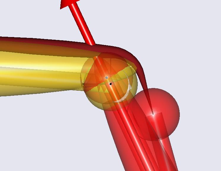
When we now run the simulation and hide the blue cylinder in the knee center, we can see that the surfaces penetrate each other quite a lot, so just putting in the geometries into the model does not change anything except that the locations of the two implants are now visible.

Now, we want to make the surfaces slide along each other. Therefore, we define a contact force that pushes the surfaces apart as soon as they are in contact. We define an AnyForceSurfaceContact and place it just below the definition of the Shank. For the definition an AnyForceSurfaceContact, we have to specify the two contacting STL surfaces (the first one is called master, the second is the slave surface) and a pressure module. This pressure module is a constant defining a linear law between penetration volume and force. In this example we use a more or less arbitrary value for this module. Our AnyForceSurfaceContact object looks like this:

  AnyRefNode Quadriceps = {
    sRel={0.05, 0.3, 0.0};
  };
}; //END of AnySeg Shank

// Define a contact force between the STL surfaces of the femoral condyle and 
// the tibial plateau to make these surfaces to make the surfaces slide along
// each other.
AnyForceSurfaceContact ContactForce = {  
  AnySurface &surfMaster = .Thigh.KneeCenter.FemoralHead;
  AnySurface &surfSlave = .Shank.KneeCenter.SurfSTLCenter.TibialPlateau;
  PressureModule = 5e7;
  ForceViewOnOff = On;
};

The AnyForceSurfaceContact creates a 3-D force vector located in the center of pressure whenever the volumes defined by the STL files penetrate each other. If the volumes are not penetrating, these forces just become zero.

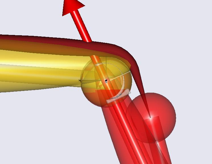
Running the simulation now shows that the tibial plateau slides along the femoral condyle and the reference frames defined in the knee centers stay close to each other with minmal penetration.

You will experience that the simulation takes longer to run now. When running simulations like this one, we can encounter that in many steps the system cannot be solved with the requested error tolerance. The reason for this problem is that small changes in the position can result in big changes in the contact force. Possibilities to improve this behavior are to exchange the surface geometries and use finer meshes or to use a softer contact by reducing the PressureModule.

We are now done with this lesson. You can now play around with this model by changing e.g. the pressure module to change the penetration of the implants or the positions of the tibial part to change the motion. If you couldn’t make your model run up to this point, you can find the complete model here.

In Lesson5 we can see how this kind of joint can be included into an existing model based on an AMMR body model.